GPU basics: from hardware architecture to AI compute
A systematic view of GPU hardware architecture, the CUDA programming model, memory hierarchy, and compute units, as the foundation for deeper AI Infra work
The GPU is the “engine” of the large-model era. Training a hundred-billion-parameter LLM can take thousands of GPUs running for months, and inference throughput and latency also track how well you use the GPU. For an AI Infra engineer, understanding GPUs is not optional; it is the hardware base for every later optimization (kernels, parallelism, scheduling).
This article starts from the basic questions: why are GPUs a fit for AI compute? What does the inside look like? How does a program run on one? The goal is a complete mental model of the GPU.
Table of contents
- 1. CPU vs GPU: why deep learning chose the GPU
- 2. GPU hardware architecture
- 3. Memory hierarchy and bandwidth
- 4. Tensor Core: the core engine of AI acceleration
- 5. The CUDA programming model
- 6. Key GPU performance metrics
- 7. Mainstream AI GPUs side by side
- 8. Memory management: a core AI Infra challenge
- 9. Multi-GPU interconnect: from one node to a cluster
- Summary
- Self-check list
- References
1. CPU vs GPU: why deep learning chose the GPU
The best way to see the value of a GPU is to put it next to a CPU.
Imagine grading 10,000 multiple-choice exams. The CPU approach hires one experienced grader: fast, can handle hard problem types, but one paper at a time. The GPU approach hires 10,000 temps who only know how to match answer keys, but they all start at once and finish in a second.
That is the core difference between latency-oriented and throughput-oriented design.
1.1 A fundamental difference in architecture philosophy
| 📊 Dimension | CPU | GPU |
|---|---|---|
| Design goal | Low latency on complex tasks | High throughput on many simple tasks |
| Core count | A few to tens of “big cores” | Thousands to tens of thousands of “small cores” |
| Per-core capability | Strong (complex branch prediction, out-of-order exec) | Weak (simple ALU, in-order) |
| Cache share | Most of the die area | A small part of the die |
| Control logic | Complex (OoO, branch predictors) | Simple (many cores share control) |
| Memory bandwidth | Lower (DDR5 ~100 GB/s) | Very high (HBM3 ~3 TB/s) |
| Best fit | Serial logic, OS, network services | Matrix math, data parallel, graphics |
1.2 Why deep learning fits GPUs naturally
What is the compute core of deep learning? At the bottom it is massive matrix multiply and element-wise ops:
- Forward: every layer is , matrix multiply at heart
- Backward: gradients are still matrix multiply ()
- Attention: , still matrix multiply at the core
These ops share two traits:
- Very high data parallelism: each element’s work is independent and maps cleanly onto different compute cores
- Regular compute patterns: little complex branching; all threads run the same instructions
That is exactly what GPUs are good at: thousands of simple cores at once, with throughput far beyond a CPU.
💡 Tip: One H100 GPU delivers about 989 TFLOPS of FP16. A high-end server CPU (such as Intel Xeon w9-3595X) usually sits in the single-digit TFLOPS for FP16. The gap is more than two orders of magnitude.
2. GPU hardware architecture
Once you know why GPUs are fast, look at what the inside looks like. Taking NVIDIA GPUs as the example, outside-in there are three layers:
2.1 The GPC → TPC → SM hierarchy
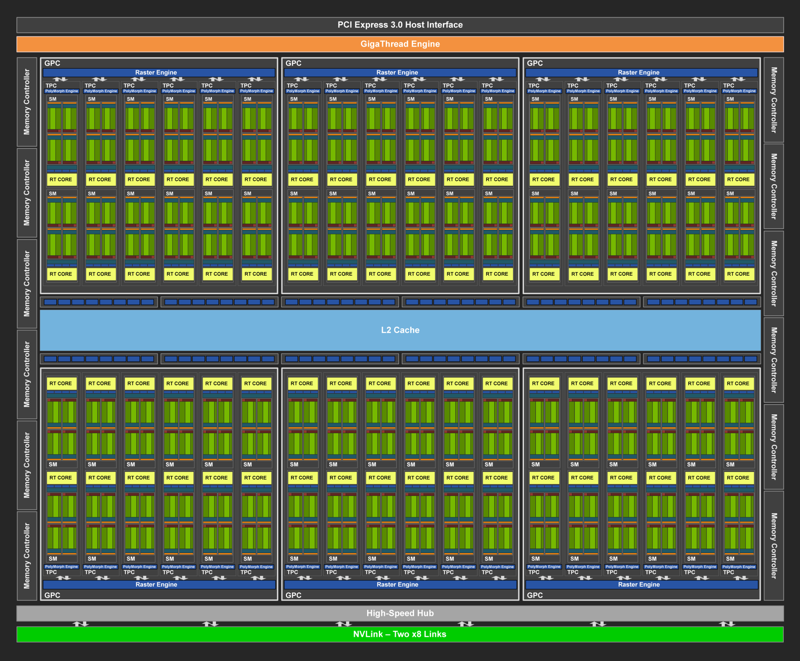
NVIDIA GPU compute cores are organized hierarchically, a bit like a large company org chart:
GPU chip
├── GPC (Graphics Processing Cluster)  ← "business unit"
│   ├── TPC (Texture Processing Cluster)  ← "department"
│   │   ├── SM (Streaming Multiprocessor)  ← "team"; basic GPU scheduling unit
│   │   │   ├── CUDA Core × N  ← "staff"; FP32/INT32 math
│   │   │   ├── Tensor Core × M  ← "specialists"; matrix math
│   │   │   ├── SFU (Special Function Unit)  ← sin/cos/exp and similar
│   │   │   ├── Register File  ← register file (fastest storage)
│   │   │   ├── Shared Memory  ← shared by all threads in the SM
│   │   │   └── L1 Cache
│   │   └── SM ...
│   └── TPC ...
├── GPC ...
├── L2 Cache (global, shared)
└── Memory Controller → HBM (device memory)
2.2 SM: the basic scheduling unit of the GPU
The SM (Streaming Multiprocessor) is the key to GPU architecture. All thread scheduling and execution happen at the SM level.
On an H100 SM, for example, each SM contains:
| 🔧 Component | Count | Role |
|---|---|---|
| CUDA Core (FP32) | 128 | Floating-point and integer ops |
| Tensor Core (4th gen) | 4 | Matrix multiply-accumulate (MMA) |
| Load/Store Unit | 32 | Memory reads and writes |
| SFU | 16 | Transcendentals (sin, cos, exp, …) |
| Warp Scheduler | 4 | Schedules 4 warps per cycle |
| Register File | 256 KB | Per-thread private registers |
| Shared Memory / L1 Cache | 228 KB (configurable) | Fast storage shared inside the SM |
📌 Key point: The SM is the smallest resource-allocation grain. When you write a CUDA kernel, a Thread Block is scheduled onto one SM. Registers, shared memory, and other SM resources are shared by all Thread Blocks on that SM.
2.3 Warp: the smallest execution unit on the GPU
GPUs do not run one thread at a time. They run in warps: 32 threads lock-step on the same instruction. Like a marching squad: 32 soldiers hear one command and step with the same foot.
Warp (32 threads)
├── Thread 0:  execute add r1, r2, r3
├── Thread 1:  execute add r1, r2, r3  (same instruction, different data)
├── Thread 2:  execute add r1, r2, r3
├── ...
└── Thread 31: execute add r1, r2, r3
This execution model is SIMT (Single Instruction, Multiple Threads), NVIDIA’s extension of SIMD.
⚠️ Note: If threads inside a warp hit a branch (if-else), threads on different paths are masked, so some sit idle. That is warp divergence, a performance killer you should avoid hard in GPU programming.
3. Memory hierarchy and bandwidth
Fast compute is useless if data cannot be fed. In AI workloads, memory bandwidth often becomes the bottleneck before raw FLOPS. That is why AI Infra people say “Memory is the new compute”.
3.1 The GPU storage hierarchy pyramid
GPU storage, like the CPU’s, gets faster and smaller as you get closer to the compute cores. The table below uses H100 SXM; bandwidths are full-GPU aggregate:
| 📊 Level | Capacity | Bandwidth | Latency | Scope | Notes |
|---|---|---|---|---|---|
| Register | ~255 per thread | — | ~0 cycle | Private to one thread | Fastest; very limited capacity |
| Shared Memory | ~228 KB per SM | ~31 TB/s | ~30 cycle | All threads in the SM | Programmer-managed “L1-class” cache |
| L1 Cache | Shared with Shared Memory | Combined with Shared Memory ~31 TB/s | ~30 cycle | Inside the SM | Hardware-managed |
| L2 Cache | ~50 MB per GPU | ~9.45 TB/s | ~200 cycle | Global | Shared by all SMs |
| HBM (device memory) | 80 GB | 3.35 TB/s | ~600 cycle | Global | Main store; bandwidth caps throughput |
Bandwidth notes:
- Shared Memory ~31 TB/s is a theoretical estimate: 32 banks per SM × 4 B/cycle = 128 B/cycle, so 132 SM × 128 B × 1.83 GHz ≈ 31 TB/s, assuming no bank conflicts.
- L1 and Shared Memory are the same physical SRAM and share bandwidth. The 30.92 TB/s in the TileLang paper is the combined figure; do not treat it as L1 alone.
- L2’s 9.45 TB/s is from Table 2 in Appendix D of the TileLang paper. Measured L2 values vary a lot by method; treat this as an order-of-magnitude reference.
- HBM3’s 3.35 TB/s is NVIDIA’s official theoretical peak.
3.2 HBM: high-bandwidth memory
Classic GDDR is like a single-lane road: limited transfer rate. HBM (High Bandwidth Memory) stacks thousands of lanes, connects to the GPU die through a silicon interposer, and multiplies bandwidth.
| 📊 Memory type | Example GPU | Bandwidth | Capacity |
|---|---|---|---|
| GDDR6X | RTX 4090 | 1,008 GB/s | 24 GB |
| HBM2e | A100 | 2,039 GB/s | 80 GB |
| HBM3 | H100 | 3,350 GB/s | 80 GB |
| HBM3e | B200 | 8,000 GB/s | 192 GB |
💡 Tip: From A100 to B200, memory bandwidth grew nearly 4×. That matters a lot for LLM inference: decode is a classic memory-bound phase, so roughly doubling bandwidth roughly doubles theoretical throughput.
3.3 The Roofline model: balancing FLOPS and bandwidth
To tell whether a task is compute-bound or memory-bound, use arithmetic intensity:
When arithmetic intensity is below the GPU’s ops:byte ratio (FLOPS / bandwidth), the task is memory-bound; otherwise it is compute-bound.
For H100 SXM:
- FP16 compute: 989 TFLOPS
- HBM3 bandwidth: 3,350 GB/s
- ops:byte ratio = FLOPs/Byte
Meaning: for every byte your kernel reads from device memory, you need at least 295 FP16 FLOPs to keep the compute busy. Otherwise the GPU sits waiting on data.
📌 Key point: Most deep-learning operators (especially Attention, LayerNorm, activations, and similar) sit far below 295 arithmetic intensity. That is why FlashAttention, kernel fusion, and similar techniques matter so much: the core idea is less memory traffic and higher arithmetic intensity.
4. Tensor Core: the core engine of AI acceleration
CUDA Cores run scalar arithmetic. Take an execution unit that can do one FP32 FMA (fused multiply-add) per cycle: peak throughput is 2 FLOPs per cycle. Tensor Cores are units built for matrix multiply-accumulate; each cycle they can do many scalar multiply-add equivalents. Exact throughput depends on architecture, input precision, accumulate precision, and whether structured sparsity is used.
4.1 How it works
The basic Tensor Core op is matrix multiply-accumulate (MMA):
, , , and are small matrices (exact shapes depend on precision and architecture generation).
For the PTX instruction mma.sync.aligned.m16n8k16.row.col.f32.f16.f16.f32, is the logical matrix shape :
- Matrix A: shape 16 × 16, FP16.
- Matrix B: shape 16 × 8, FP16.
- Matrices C and D: shape 16 × 8, FP32, for accumulate and output.
- One full MMA does FLOPs, counting one scalar multiply-add as 2 FLOPs.
Instruction shape is not the same as one Tensor Core’s per-cycle throughput. The mma.sync above is executed cooperatively by a whole warp; 4096 FLOPs is the total for that warp-level op. Do not multiply by 32 again, and do not treat it as what one Tensor Core finishes in one cycle. PTX describes instruction semantics; hardware throughput and latency need the target architecture docs and cannot be deduced from alone. NVIDIA PTX ISA: mma
4.2 Evolution of precision formats
Different formats trade compute, accuracy, and memory differently:
| 📊 Precision | Bit width | Dynamic range | First Tensor Core support | Typical use |
|---|---|---|---|---|
| FP32 | 32 bit | High | — | Baseline precision, loss accumulation |
| TF32 | 19 bit | Same as FP32 | Ampere (A100) | Training (default FP32 path on Ampere) |
| FP16 | 16 bit | Narrower | Volta (V100) | Mixed-precision training (needs loss scaling) |
| BF16 | 16 bit | Same as FP32 | Ampere (A100) | Mixed-precision training (preferred; no loss scaling) |
| FP8 (E4M3/E5M2) | 8 bit | Selectable | Hopper (H100) | Training + inference |
| INT8 | 8 bit | Integer | Turing (T4) | Inference quantization |
| FP4 | 4 bit | Very narrow | Blackwell (B200) | Inference quantization |
💡 Tip: BF16 and FP16 are both 16-bit, but BF16 keeps the same 8-bit exponent as FP32, so the dynamic range is larger and training overflows less easily. Modern large-model training almost always uses BF16 rather than FP16.
4.3 Tensor Core compute multipliers
Peak numbers differ a lot by compute path. For H100 SXM, the table uses dense numbers; Tensor Core rows use FP32 accumulate:
| 📊 Compute path | Theoretical peak (approx.) |
|---|---|
| CUDA Core, FP32 FMA | 67 TFLOPS |
| Tensor Core, TF32 input | 495 TFLOPS |
| Tensor Core, FP16 / BF16 input | 989 TFLOPS |
| Tensor Core, FP8 input | 1,979 TFLOPS |
These are hardware peaks for different precisions and paths, not application speedups. TF32 in particular does not have full FP32 mantissa precision. Starred Tensor Core numbers on the NVIDIA H100 product page include sparsity; the table above divides those by 2 for an approximate dense value. NVIDIA H100 specs and sparsity footnotes
📌 Key point: To trigger Tensor Core acceleration, matrix dimensions must meet alignment rules (usually multiples of 8 or 16). In practice, if a model’s hidden_size is not a multiple of 8, Tensor Cores may be underused.
5. The CUDA programming model
CUDA is NVIDIA’s parallel compute framework and the bridge between software algorithms and hardware execution. Even if you live in PyTorch and rarely write CUDA by hand, understanding the programming model helps you see what happens underneath.
5.1 Thread hierarchy: Grid → Block → Thread
CUDA programs run on the GPU as kernels. Kernel threads are organized in three levels:
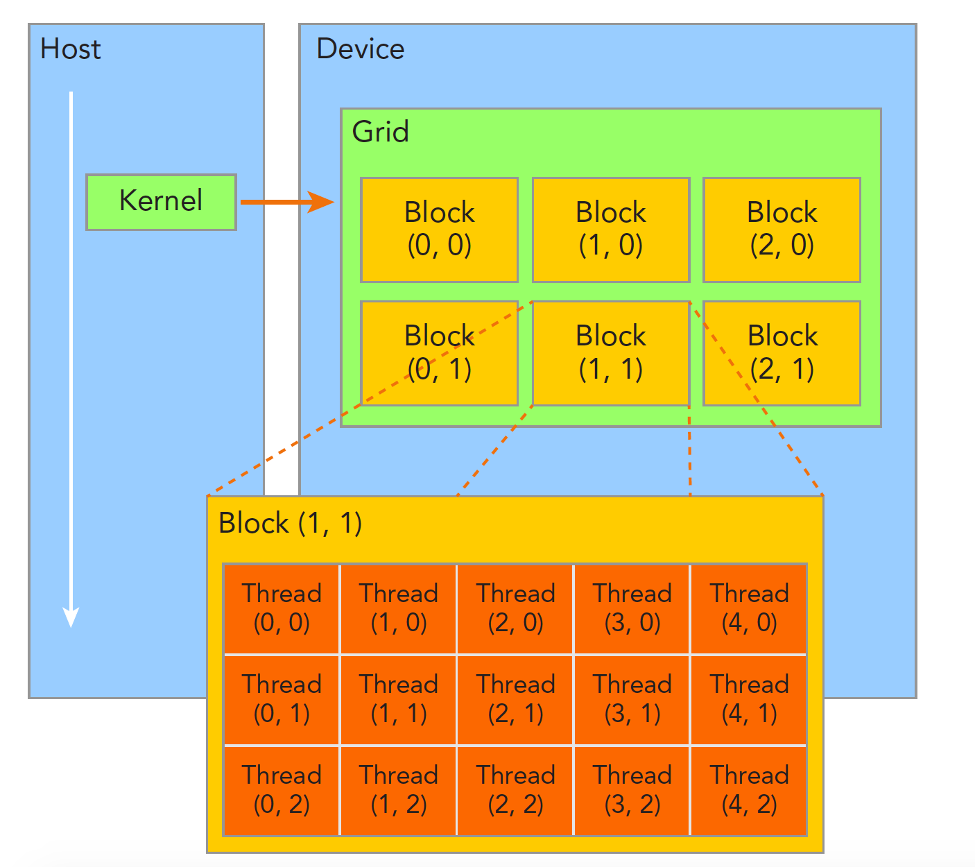
| 📊 Level | Meaning | Hardware mapping |
|---|---|---|
| Grid | All threads of one kernel launch | Whole GPU |
| Block | A cooperating group of threads (up to 1024) | Scheduled onto one SM |
| Thread | Smallest execution unit | CUDA Core |
| Warp | 32 consecutive threads (implicit grouping) | Warp Scheduler in the SM |
5.2 A simple CUDA kernel example
A vector-add CUDA kernel that shows the basic pattern:
// Vector add kernel: C[i] = A[i] + B[i]
__global__ void vecAdd(float *A, float *B, float *C, int N) {
    // Global index this thread owns
    int idx = blockIdx.x * blockDim.x + threadIdx.x;

    // Bounds check
    if (idx < N) {
        C[idx] = A[idx] + B[idx];
    }
}

// Host-side kernel launch
int main() {
    int N = 1000000;
    int threadsPerBlock = 256;
    int blocksPerGrid = (N + threadsPerBlock - 1) / threadsPerBlock;

    // <<<grid dim, block dim>>>
    vecAdd<<<blocksPerGrid, threadsPerBlock>>>(d_A, d_B, d_C, N);
    return 0;
}
Execution flow: 📥 Host allocates device memory and copies data → ⚙️ launches the kernel; the GPU assigns blocks to SMs → 📤 kernel finishes; results copy back to the host.
5.3 Memory model and storage mapping
Different CUDA variable declarations map to different hardware stores:
| 📊 CUDA memory type | How you declare it | Hardware location | Scope | Lifetime |
|---|---|---|---|---|
| Register | Local variable | SM register file | One thread | Kernel |
| Local Memory | Spilled local variables | HBM (device memory) | One thread | Kernel |
| Shared Memory | __shared__ | On-chip SM storage | Inside a block | Kernel |
| Global Memory | __device__ / cudaMalloc | HBM (device memory) | All threads | Application |
| Constant Memory | __constant__ | HBM + cache | All threads | Application |
⚠️ Note: Despite the name, Local Memory lives in HBM and is as slow as Global Memory. When registers run out, the compiler spills variables to Local Memory. That is register spilling, a performance issue to watch for.
5.4 Feeling GPU compute through PyTorch
Most AI Infra engineers do not write CUDA C daily; they call it indirectly through frameworks like PyTorch. Understanding CUDA underneath still helps you write faster PyTorch:
import torch
import time

# Check GPU info
if torch.cuda.is_available():
    gpu = torch.cuda.get_device_properties(0)
    print(f"GPU: {gpu.name}")
    print(f"SM count: {gpu.multi_processor_count}")
    print(f"Memory: {gpu.total_memory / 1024**3:.1f} GB")

# CPU vs GPU matmul performance
N = 4096
A_cpu = torch.randn(N, N)
B_cpu = torch.randn(N, N)
A_gpu = A_cpu.cuda()
B_gpu = B_cpu.cuda()

# Warmup
torch.mm(A_gpu, B_gpu)
torch.cuda.synchronize()

# Timing
start = time.perf_counter()
C_cpu = torch.mm(A_cpu, B_cpu)
cpu_time = time.perf_counter() - start

torch.cuda.synchronize()
start = time.perf_counter()
C_gpu = torch.mm(A_gpu, B_gpu)
torch.cuda.synchronize()
gpu_time = time.perf_counter() - start

print(f"CPU: {cpu_time*1000:.2f} ms | GPU: {gpu_time*1000:.2f} ms | Speedup: {cpu_time/gpu_time:.1f}x")
6. Key GPU performance metrics
To judge a GPU’s AI compute capability, watch these core metrics:
6.1 Four core metrics
| 📊 Metric | Meaning | Why it matters |
|---|---|---|
| Compute (TFLOPS) | Floating-point ops per second | Caps compute-bound work |
| Memory bandwidth (GB/s) | Bytes read/written to device memory per second | Caps memory-bound work |
| Memory capacity (GB) | Total data you can store | Caps how large a model you can run |
| Interconnect bandwidth (GB/s) | GPU-to-GPU communication speed | Caps multi-GPU scaling efficiency |
6.2 Peak compute formulas
Before quoting a theoretical peak, pin down GPU model, execution path, input and accumulate precision, dense vs sparse accounting, and clock. Saying only “FP16 FLOPS” is not enough; CUDA Core and Tensor Core FP16 throughput differ.
General formula: number of units × FLOPs per unit per cycle × cycles per second.
- : number of SMs actually enabled on that GPU.
- : number of chosen compute units per SM.
- : FLOPs each unit can finish per cycle at the chosen precision and mode, in FLOPs/(unit·cycle).
- : core clock matching that throughput spec, in Hz; result is FLOP/s; divide by for TFLOPS. Do not use memory clock, and do not plug in a max frequency that does not apply to that execution path.
CUDA Core: the ×2 is the FMA counting convention. One scalar FMA () counts as one multiply plus one add, i.e. 2 FLOPs. That does not mean every unit only ever does 2 FLOPs per cycle. If an FP32 unit peaks at one scalar FMA per cycle, ; for FP16, FP64, or other instructions, look up that architecture’s throughput again. A half2 instruction can express two FP16 elements, but the per-cycle issue rate still depends on hardware; you cannot blanket-estimate with “FP16 core count × 2”. CUDA Programming Guide: arithmetic instruction throughput
Tensor Core: you must count multiple multiply-adds per cycle. Let be the number of scalar FMA equivalents one Tensor Core finishes per cycle. Dense peak is:
Here is sustained hardware throughput. Do not replace it with an MMA’s , and do not take the reciprocal of a single instruction’s latency; the pipeline can overlap independent ops. If a source already gives FLOPs/cycle, the ×2 for multiply-add is already included; do not multiply again.
Worked example: A100 FP16 input, FP32 accumulate, dense Tensor Core peak. The NVIDIA whitepaper gives A100 108 SMs with 4 Tensor Cores each; each Tensor Core finishes 256 FP16 multiply-adds per cycle, i.e. FLOPs. Using the 1.41 GHz Boost clock from the spec table:
On the same A100, the ordinary FP32 path has 64 FP32 CUDA Cores per SM. Counting one FMA per unit per cycle and converting units gives TFLOPS. Together they show why counting “cores” or looking only at bit width cannot compare compute. NVIDIA A100 Architecture Whitepaper, pp. 20, 24 and the spec table
Keep sparse peaks separate from measured performance. When A100 meets 2:4 structured sparsity and uses the matching sparse Tensor Core instructions, the FP16 dense-equivalent peak reaches about 624 TFLOPS, 2× the dense peak above. That number counts ops as if for an equivalent dense matrix; ordinary dense matrices or arbitrarily placed zeros do not get the boost automatically. When reading vendor specs, check whether each number says “with sparsity”; do not assume every TFLOPS figure includes sparsity. NVIDIA Ampere architecture deep dive
Actual throughput should be computed as “work finished / measured time,” e.g. dense GEMM often estimated as , then compared to a peak with the same precision, path, and counting rules. Matrix shape, memory traffic, instruction mix, parallelism, and frequency changes from power/thermal all affect utilization. There is no universal “30%–60% of peak” band. GPU compute is asynchronous; timing also needs correct sync or CUDA Events.
7. Mainstream AI GPUs side by side
Core specs for mainstream NVIDIA AI GPUs as of 2025:
| 📊 Model | Architecture | SM count | Memory | Bandwidth | FP16 compute | FP8 compute | TDP | Typical use |
|---|---|---|---|---|---|---|---|---|
| V100 | Volta | 80 | 32 GB HBM2 | 900 GB/s | 125 TFLOPS | — | 300W | Classic training card |
| A100 SXM | Ampere | 108 | 80 GB HBM2e | 2,039 GB/s | 312 TFLOPS | — | 400W | Training + inference |
| H100 SXM | Hopper | 132 | 80 GB HBM3 | 3,350 GB/s | 989 TFLOPS | 1,979 TFLOPS | 700W | Large-scale training |
| H200 | Hopper | 132 | 141 GB HBM3e | 4,800 GB/s | 989 TFLOPS | 1,979 TFLOPS | 700W | Long-sequence inference |
| B200 | Blackwell | 160 | 192 GB HBM3e | 8,000 GB/s | 2,250 TFLOPS | 4,500 TFLOPS | 1000W | Next-gen flagship |
| L40S | Ada | 142 | 48 GB GDDR6 | 864 GB/s | 366 TFLOPS | — | 350W | Inference / multimedia |
⚠️ Note: The same architecture can ship as SXM or PCIe. SXM usually has higher power, higher clocks, and NVLink, and is clearly stronger than PCIe. Always confirm the package when you choose hardware.
8. Memory management: a core AI Infra challenge
When training large models, memory is often the first wall you hit. A 7B model in FP16 needs about 14 GB for parameters alone; add optimizer state, gradients, and activations and real usage can reach 4–8× the parameter size.
8.1 Where training memory goes
With Adam + FP16 mixed precision, memory per parameter:
| 📊 Component | Bytes per param | Notes |
|---|---|---|
| FP16 parameters | 2 B | Used in forward / backward |
| FP32 parameter copy | 4 B | Adam keeps FP32 master weights |
| FP32 gradients | 4 B | Produced by backward |
| Adam first moment (m) | 4 B | EMA of gradients |
| Adam second moment (v) | 4 B | EMA of squared gradients |
| Total | 18 B | — |
Fixed memory for a 7B model = GB, not counting activations.
8.2 Common memory optimization strategies
Facing “not enough memory,” AI Infra has a set of classic strategies:
| 📊 Strategy | Idea | Memory saved | Cost |
|---|---|---|---|
| Mixed-precision training | FP16/BF16 for forward/backward; FP32 for updates | ~50% of parameter memory | Needs loss scaling (FP16) |
| Gradient accumulation | Accumulate grads over micro-batches; emulate a large batch | Lower activation peaks | More training steps |
| Gradient checkpointing | Keep only some activations in forward; recompute in backward | Activation memory down to | ~33% more compute |
| ZeRO | Shard optimizer state / gradients / parameters across GPUs | Linear drop in per-GPU memory | More communication |
| Offloading | Move some state to CPU memory or NVMe | Break the single-GPU memory ceiling | PCIe bandwidth becomes the limit |
💡 Tip: These strategies are not mutually exclusive; practice usually combines them. DeepSpeed ZeRO Stage 2 + mixed precision + gradient checkpointing is a common setup for mid-to-large models (7B–70B).
9. Multi-GPU interconnect: from one node to a cluster
When one GPU’s memory and compute are not enough, you go multi-GPU. Interconnect bandwidth and topology directly set how well parallel training scales.
9.1 Interconnect comparison
| 📊 Interconnect | Bandwidth | Scenario | Notes |
|---|---|---|---|
| PCIe 5.0 | 128 GB/s (bidirectional) | Cross-GPU (general) | Ubiquitous but lower bandwidth |
| NVLink 4.0 (Hopper) | 900 GB/s (full duplex) | Intra-node GPU links | Dedicated high-speed; used on H100 |
| NVLink 5.0 (Blackwell) | 1,800 GB/s (full duplex) | Intra-node GPU links | Used on B200 |
| NVSwitch | Connects all NVLink | Full mesh inside a node | All-to-all at full bandwidth |
| InfiniBand NDR | 400 Gb/s (50 GB/s) | Cross-node | Standard for large clusters |
9.2 Typical multi-GPU topology
On a DGX H100 (8 GPUs), for example:
- 8 H100s are fully connected through NVSwitch; any pair has 900 GB/s
- Each machine joins the cluster through 8 ConnectX-7 InfiniBand NICs
- Intra-node >> inter-node bandwidth; that gap shapes parallelism strategy
📌 Key point: When designing distributed training, put high-traffic dimensions (such as tensor parallelism) on high-bandwidth intra-node NVLink, and lower-traffic dimensions (data parallel, pipeline parallel) on inter-node InfiniBand.
# Inspect GPU topology
nvidia-smi topo -m

# Inspect NVLink status
nvidia-smi nvlink -s
📝 Summary
Starting from CPU vs GPU architecture differences and moving into the GPU’s internal structure, this article covered:
- Why GPUs: deep learning’s matrix math fits GPU massively parallel hardware
- Hardware architecture: GPC → TPC → SM → CUDA Core / Tensor Core; warp is the smallest scheduling unit
- Memory hierarchy: Register → Shared Memory → L1/L2 Cache → HBM; bandwidth often bottlenecks before FLOPS
- Tensor Core: MMA units built for matrix multiply-accumulate; lower-precision formats like BF16/FP8 keep pushing compute up
- CUDA programming model: Grid → Block → Thread organization, and how memory types map to hardware
- Performance evaluation: the four core metrics: compute, bandwidth, memory capacity, interconnect bandwidth
- Memory management: mixed precision, gradient accumulation, checkpointing, ZeRO, and related classics
- Multi-GPU interconnect: NVLink, NVSwitch, and InfiniBand form the path from one node to a cluster
With this base you have the hardware context to read later articles on CUDA programming, distributed training, and inference optimization.
🎯 Self-check list
- Can state the core architectural difference between CPU and GPU design philosophy
- Can sketch the GPU hierarchy (GPC → SM → CUDA Core / Tensor Core)
- Can explain warps and why warp divergence hurts performance
- Can state capacity and speed order of magnitude for Register → Shared Memory → L2 → HBM
- Can use the Roofline model to judge whether an operator is compute-bound or memory-bound
- Can explain BF16 vs FP16 and why large-model training prefers BF16
- Can list three or more memory optimization strategies and their ideas
- Can use
nvidia-smito inspect GPU status and topology - Can state the order-of-magnitude bandwidth gap between NVLink and PCIe
- Can estimate memory for a 7B model trained with Adam + FP16 mixed precision
📚 References
- NVIDIA CUDA C++ Programming Guide
- NVIDIA H100 Tensor Core GPU Architecture Whitepaper
- NVIDIA A100 Tensor Core GPU Architecture Whitepaper
- NVIDIA Blackwell Architecture Whitepaper
- Mixed Precision Training - NVIDIA Developer Blog
- ZeRO: Memory Optimizations Toward Training Trillion Parameter Models
- Roofline: An Insightful Visual Performance Model