🔥 Transformer architecture: a quick start
Understand the full Transformer from an AI Infra engineer's view: Self-Attention, FFN, positional encoding, and what each module means in practice
Transformer is the common base of the large-model era. The CUDA layer optimizes its operators, the distributed layer shards its parameters, and the inference layer speeds up its generation. This article takes an AI Infra engineer’s view of what that “thing every later optimization acts on” actually looks like, why it looks that way, and which later optimizations keep coming back to each module.
📑 Contents
- 1. Why AI Infra engineers need to understand Transformer
- 2. The Transformer network at a glance
- 3. Self-Attention
- 4. Feed-forward network (FFN)
- 5. Positional encoding
- 6. LayerNorm and residual connections
- 7. A full Transformer Decoder Block
- 8. From Transformer to LLM: autoregressive generation
- Summary
- Self-check list
- References
1. Why AI Infra engineers need to understand Transformer
If you are going deep into AI Infra, whether writing CUDA kernels, doing distributed training, or deploying inference, the main object of your work is the same thing: the Transformer model.
It is like a car engineer who has to understand the engine. You do not need to design the engine yourself (that is the researcher’s job), but you need to know where the crankshaft is, how the pistons move, and how the oil path runs. Otherwise how would you know which part to optimize?
Concretely, each layer of AI Infra work maps straight onto some Transformer module:
| AI Infra layer | Core work | Matching Transformer module |
|---|---|---|
| CUDA operator optimization | FlashAttention, efficient GEMM kernels | /PV matmul in Self-Attention |
| CUDA operator optimization | Fused Softmax, Online Softmax | Softmax in Attention |
| CUDA operator optimization | LayerNorm kernel fusion | Normalization in each Block |
| Distributed training | Tensor Parallelism | Multi-head split in Attention, matrix split in FFN |
| Distributed training | Pipeline Parallelism | Stacked multi-layer Decoder Blocks |
| Distributed training | ZeRO memory optimization | Storage and communication of every parameter matrix |
| Inference deployment | KV Cache management | K and V matrices in Self-Attention |
| Inference deployment | PagedAttention | KV Cache fragmentation in GPU memory |
| Inference deployment | Quantization (INT4/INT8/FP8) | All weight matrices and the KV Cache |
One-line takeaway: if you do not understand Transformer, you do not know what you are optimizing. Every optimization technique you meet later can be traced back to a concrete module in this article.
2. The Transformer network at a glance
Before taking the modules apart one by one, look at the Transformer as a whole, the way you would glance at an assembly drawing before tearing an engine down: which parts exist, and how they connect.
2.1 The original Transformer: Encoder-Decoder
The original Transformer from the 2017 paper “Attention Is All You Need” has two main parts:
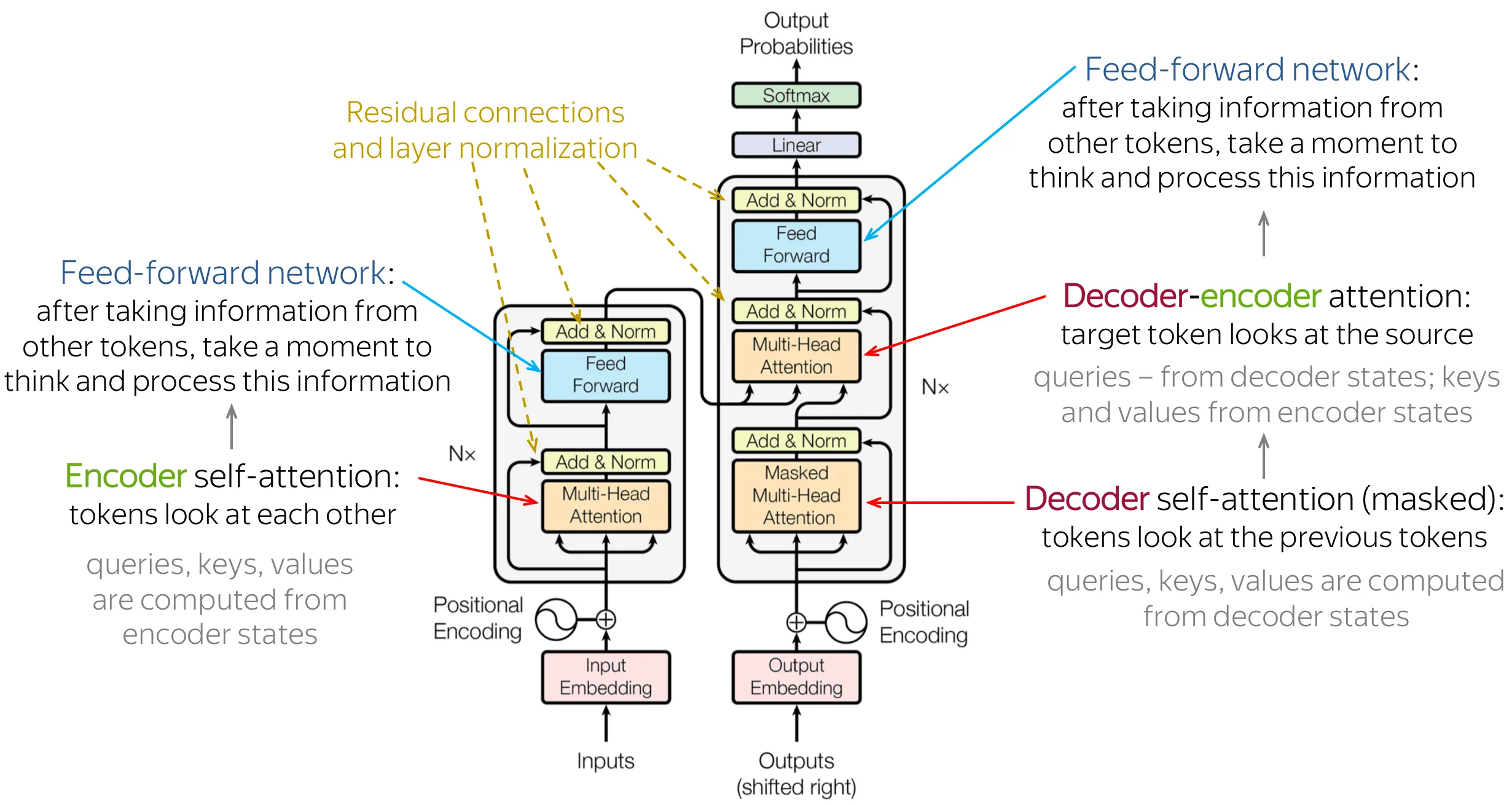
- Encoder: reads the input sequence and builds a contextual representation. Each layer has one Self-Attention and one FFN; every token can attend to every other token (bidirectional attention)
- Decoder: generates the target sequence autoregressively from the Encoder output. Each layer has a causally masked Self-Attention (only already generated tokens), a Cross-Attention (over Encoder outputs), and an FFN
This Encoder-Decoder design was built for machine translation: the Encoder understands the source language, the Decoder generates the target language.
2.2 What large models use today: Decoder-only
The success of the GPT series showed a useful fact: a Decoder alone is enough. Almost every mainstream large language model today (GPT, LLaMA, Mistral, Qwen, DeepSeek) uses a Decoder-only architecture. The Encoder and Cross-Attention are gone; what remains is causally masked Self-Attention.
The overall structure is three stages: input layer, a stack of N Decoder Blocks, output layer:
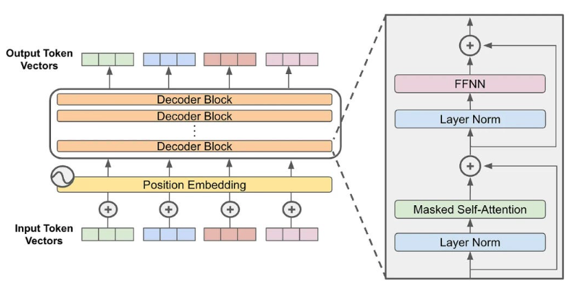
The model’s core is that middle stack of N Decoder Blocks. Every Block has the same structure and two submodules:
- Masked Self-Attention: each token aggregates information from earlier tokens (section 3)
- FFN: a nonlinear transform applied independently to each token (section 4)
Each submodule is preceded by LayerNorm (section 6) and followed by a residual connection that adds the submodule input back (section 6). Position information is injected via RoPE during the Attention compute (section 5).
You may wonder why the Decoder block in this Decoder-only setup differs from the Decoder block in Encoder-Decoder. That is the Pre-Norm vs Post-Norm difference covered later.
2.3 Three architecture variants
| Architecture | Representative models | Attention pattern | Typical uses |
|---|---|---|---|
| Encoder-only | BERT, RoBERTa | Bidirectional (every token sees every token) | Text classification, NER, information extraction |
| Encoder-Decoder | T5, BART, original Transformer | Bidirectional Encoder + causal Decoder + Cross-Attention | Translation, summarization, Seq2Seq |
| Decoder-only | GPT, LLaMA, Mistral, Qwen | Causal attention (each token sees only earlier tokens) | Text generation, chat, code generation |
Decoder-only became the mainstream choice for large models for two main reasons:
- A single training objective: every task can be cast as “predict the next token”; you do not need a different architecture per task
- Engineering simplicity: one Block shape; KV Cache management and parallel strategies at inference time stay simpler
Everything that follows in this article is about the Decoder-only architecture, the structure AI Infra engineers deal with most often.
3. Self-Attention
Self-Attention is the core of the Transformer, and also the module that burns the most compute and memory. Almost every heavy AI Infra optimization (FlashAttention, KV Cache, tensor parallelism) orbits around it.
3.1 Intuition: what Attention does
Start from a real language problem:
Sentence A: The bank of the river. (riverbank) Sentence B: Money in the bank. (financial bank)
The same word “bank” means two different things. How does a machine translation system decide? It looks at the other words: in A, “river” gets the highest weight; in B, “money” does. That mechanism of letting each word attend to the others and aggregating meaning by relevance weights is Self-Attention.
In plain terms: Attention lets every word in a sentence “look at” every other word, then aggregates information by how much attention it pays, so each word gets a new meaning fused with context.
Push the analogy further with a search. When you look up “apple” in an encyclopedia, you form a query (Query): “what is an apple?”, you scan each page’s title (Key) for relevance, and you combine the body text (Value) of the relevant pages by how relevant they are. Attention does the same thing:
- Query (Q): what I want to look up: the information the current word wants
- Key (K): index / title: how each word presents itself to be matched
- Value (V): the actual content passed on once a match succeeds
In Self-Attention, every token in the sequence plays all three roles at once: it asks (produces Q), it is an index being queried (produces K), and it provides information (produces V). Matching Q against K yields attention weights; a weighted sum of V with those weights aggregates the information.
💡 Tip: Disambiguating “bank” vs “riverbank” in the RNN era meant pushing earlier word information forward one step at a time. Self-Attention lets every word compare with every other word in the same step, so long-range dependencies no longer fade away.
3.2 The compute path: from input to output
Suppose we have a sequence of length , each token a -dimensional vector, so the input matrix has shape .
Step 1: linear projections to Q, K, V
Multiply X by three weight matrices to get Query, Key, and Value:
Here , , and each output is .
, , and are learnable parameter matrices, each of shape . Those three matmuls are three GEMM ops, and they are among the main targets of later CUDA and tensor-parallel work.
Step 2: attention scores
Use the inner product of Q and K to measure how well each pair of tokens matches:
is an matrix; is how much token attends to token (raw score).
Step 3: scale
Divide the scores by ( is the per-head dimension; more on that later):
Why scale? When is large, the Q·K inner products get large (you are summing terms), so softmax inputs differ wildly. Softmax is very sensitive to large values: once the gap grows, the output polarizes toward a near one-hot distribution, gradients collapse toward zero, and training stalls. Dividing by pulls the variance back near 1 so softmax sits in a healthier gradient range.
Step 4: Softmax
Softmax each row so raw scores become a probability distribution (each row sums to 1):
is now the attention weight token assigns to token ; each row sums to 1.
AI Infra note: Softmax looks simple, but it needs careful optimization in high-performance settings. The standard implementation scans each row twice (once for the max and the sum of exps, once to normalize). Online Softmax folds that into one scan, and FlashAttention builds its fused Attention on that idea.
Step 5: weighted sum
Multiply the attention weights A by the Value matrix V:
Each token ends up with a -dimensional vector that has fused information from the other tokens it “should” attend to.
Full formula (one line)
Step 6: output projection
Finally multiply by an output projection :
maps the concatenated multi-head result back to the model’s hidden size (next section).
3.3 Why the complexity is
The bottleneck falls straight out of the steps above.
The critical step is , shape , producing an matrix. For that step:
- Compute: : elements, each needing multiply-adds
- Memory: : you have to store the full attention matrix
Likewise has shape and also costs .
So Self-Attention’s total complexity is , usually shortened to because is a fixed model constant.
What does that mean in practice? When sequence length grows from 2K to 128K, compute and attention-matrix memory grow by 4096×. That is why long-context support is hard.
AI Infra note: That memory bottleneck is exactly what FlashAttention was built for. The standard path writes the full attention matrix to HBM (the GPU’s high-bandwidth memory). FlashAttention uses tiling plus online softmax so each step only computes a small attention tile in on-chip SRAM and then discards it; the full matrix never goes back to HBM. Extra memory drops from to , and HBM traffic drops from to ( is SRAM size; is much smaller than ). It still grows with , but the constant shrinks a lot. Compute is unchanged; memory traffic falls sharply. That is the core idea behind memory-aware optimization.
3.4 Multi-Head Attention: why multiple heads
The description above is single-head Attention. Real Transformers use Multi-Head Attention (MHA): split Q, K, V along the feature dimension into several “heads”, run Attention independently per head, then concatenate the results.
In plain language: one head can track one kind of relation (say syntactic dependency); many heads can track many relations at once (syntax, semantics, position, and so on), like several people looking at the same problem from different angles and then combining their views.
Concretely, if the model hidden size is and the head count is , each head has dimension .
Math definition (independent projections per head): rigorously, each head owns its own learnable projection matrices , and computes:
Because the projection matrices differ per head, the 32 heads learn 32 different representation subspaces from the same input . They are not simply slicing one into 32 pieces. That is the real reason multi-head can capture many relation patterns.
Engineering view (one big GEMM): in practice, to let the GPU compute every head’s in one GEMM, the 32 matrices are concatenated along columns into one large matrix:
By block matrix multiplication, is exactly along the columns, so one large matmul plus one reshape equals 32 independent projections:
Key point: reshape is not simply cutting one unified into 32 slices. It unpacks the result of “32 head projections that GEMM stored side by side.” Math says 32 independent projections; engineering merges them into one GEMM. The two views are equivalent.
Do the same for K and V. Each head computes Attention on its own:
Then concatenate the 32 head outputs and project:
Parameter makeup of multi-head:
- : , i.e. parameters
- : , parameters
- : , parameters
- : , parameters
- Total: parameters
AI Infra note: Multi-head structure is a natural fit for tensor parallelism. The 32 heads can be split evenly across GPUs: for example 4 GPUs each handle 8 heads, so each GPU only needs 1/4 of the QKV weights and compute. That is the core idea of Megatron-LM tensor parallelism: shard the Attention module along the head dimension. After the shard you only need one AllReduce to gather each GPU’s partial results.
Variants of head layout also matter: MQA (Multi-Query Attention) shares one KV set across all heads, and GQA (Grouped-Query Attention) shares one KV set across groups of heads. Both change KV Cache size and how you shard under tensor parallelism, and both are central ideas in inference optimization.
4. Feed-forward network (FFN)
Attention handles “information exchange”: tokens pass information to each other. Exchange alone is not enough; the model also needs to process each token’s information in depth. That is the job of the Feed-Forward Network (FFN).
Analogy: Attention is a roundtable where people trade opinions; FFN is everyone going back to their desk afterward to digest those opinions and form their own judgment. The FFN applies a nonlinear transform independently per token, with no cross-token interaction.
4.1 Structure: two linear layers + an activation
A standard FFN is simple: expand, then compress, with a nonlinear activation in the middle:
Where:
- : , expands from to (usually )
- Activation: introduces nonlinearity
- : , compresses from back to
With as an example:
Note: real models such as LLaMA use the SwiGLU activation (covered below). The intermediate width is rather than a plain , so total parameter count stays roughly unchanged after adding the gate.
4.2 Parameter count: why FFN dominates the model size
Let’s run the numbers for one Transformer Block:
| Module | Parameter matrices | Parameter count |
|---|---|---|
| Attention | ||
| FFN (standard) | ||
| FFN (SwiGLU) |
Roughly, FFN has about 2× the parameters of Attention. Inside a full Transformer Block, FFN accounts for about 2/3 of the parameters.
That ratio has direct engineering consequences:
AI Infra note: Because FFN holds most of the parameters, how you shard it under tensor parallelism drives communication cost. Megatron-LM shards by columns and by rows so the intermediate result needs no AllReduce, with only one AllReduce at the end. That split exploits FFN’s expand-then-compress shape. In Mixture-of-Experts (MoE) models, FFN is further split into multiple “experts”, which adds Expert Parallelism as another parallel dimension.
4.3 Activation evolution: ReLU → GELU → SwiGLU
The activation looks like a small detail, but the choice affects training stability and final quality.
ReLU (Rectified Linear Unit)
The classic activation: simple and fast. The problem: negative inputs become exactly 0, so those neurons can “die” permanently and lose information.
GELU (Gaussian Error Linear Unit)
where is the CDF of the standard normal distribution.
Intuitively, GELU does not hard on/off like ReLU. It gives a smooth “pass probability” based on the input magnitude: larger values are more likely to pass, smaller ones are more likely to be suppressed, but they do not go fully to zero. GPT-series models and BERT both use GELU.
SwiGLU (Swish-Gated Linear Unit)
where , is the sigmoid, and is element-wise multiply.
SwiGLU is the mainstream choice in large models today (LLaMA, Mistral, and others). It adds a gating mechanism: a separate gate matrix controls how much information passes, instead of applying the same activation to every dimension. The cost is an extra matrix (so FFN goes from two matrices to three: , , ), but experiments show better quality.
AI Infra note: SwiGLU’s three-matrix layout (, , ) differs from the two-matrix standard FFN, so CUDA kernel fusion and tensor-parallel sharding need special handling. For example and can be fused into one GEMM to raise GPU utilization.
5. Positional encoding
5.1 Why Transformer needs position information
This is easy to overlook and still very important.
Look back at Self-Attention: scores every pair of tokens, then those scores weight a sum over V. Notice that the process does not care about token order at all.
Thought experiment: shuffle the three tokens in “cat chases dog” into “dog cat chases”. As long as the Q, K, V values stay the same, Attention’s result is identical. In math terms, Attention is permutation equivariant over the input sequence: however you shuffle the input, the output shuffles the same way, and each token still aggregates the same information.
Language clearly has order. “Cat chases dog” and “dog chases cat” mean different things. So we have to inject position information into the Transformer somehow.
5.2 Sinusoidal positional encoding: the original paper
“Attention Is All You Need” proposed an elegant scheme: generate a unique encoding vector for each position with sine/cosine at different frequencies, and add it directly onto the token embedding.
where is the token’s position in the sequence (), and is the dimension index.
Intuition: each dimension is a clock at a different “frequency”. Low-frequency dimensions change slowly (they separate distant positions); high-frequency ones change fast (they separate nearby positions). It is like encoding time with year-month-day-hour-minute-second: “year” changes slowest but separates large spans, “second” changes fastest but only separates small spans. Together, every position gets a unique timestamp.
Pros:
- No learnable parameters; encoding length can extend in theory
- Relative position can be recovered via linear transforms (sine/cosine addition formulas)
Limits:
- Position is “added” onto the embedding, so it can dilute through deep layers
- Hard to extrapolate well beyond lengths seen in training
5.3 RoPE (rotary positional embedding): the mainstream choice today
RoPE (Rotary Position Embedding) is the positional scheme used by almost every mainstream large model (LLaMA, Mistral, Qwen, DeepSeek, and others).
Core idea: do not inject position at the embedding layer. Instead, when computing Attention, encode position by rotating the Q and K vectors.
Concretely, treat every two adjacent dimensions of Q and K as coordinates in a 2D plane, then rotate that 2D vector by an angle that depends on the token’s position:
where is a frequency parameter similar to the sinusoidal scheme. K is rotated the same way.
The key property: after rotation, the Q·K inner product depends only on the relative position difference of the two tokens, not on absolute position. You can show:
So Attention naturally encodes relative position, which fits language understanding well (“the relation between word 3 and word 5” matters more than “the absolute positions of word 3 and word 5”).
Why RoPE became mainstream:
- Relative positional encoding; naturally handles variable-length input
- No extra parameters
- Compatible with linear Attention and related variants
- Extrapolates better than sinusoidal (with NTK-aware and other interpolation methods you can extend context length)
AI Infra note: RoPE’s rotation (element-wise multiply-add at heart) is cheap per call but frequent, so it is usually fused into the Attention kernel rather than launched as its own kernel. In long-context settings, tuning RoPE’s frequency parameters (NTK-aware Scaling, YaRN, and so on) directly affects the maximum sequence length the model can support, which ties into KV Cache management and memory planning.
6. LayerNorm and residual connections
6.1 Residual connections: keep the gradient path open
Residual connections come from ResNet and are extremely simple:
where SubLayer can be an Attention layer or an FFN layer.
Intuition: learn only the delta on top of the original information
Read a residual as: output = original information + learned change. Example:
Suppose = “the cat is on the table”, and Attention learns = “emphasize the relation between ‘cat’ and ‘table’”. Then:
means: keep the original sentence, and strengthen the semantic relation.
Why design it this way?
1️⃣ Fix hard training in deep networks
Transformers often have dozens of layers (LLaMA-2 has 32; GPT-4 is rumored to have over a hundred). Without residuals, the signal path is . During backprop the gradient is a long chain of multiplies and can shrink toward zero (vanishing gradients), so deep nets fail to train well.
With residuals the path becomes , and gradients can take a shortcut:
Because of the identity term , the gradient does not become , and training is more stable. Residuals give a “highway”: gradients can flow straight back to shallow layers along the residual path, unaffected by intermediate transforms.
2️⃣ Make identity maps easier to learn
Ideally, if a layer needs no transform, learning is enough and the output is . The network can skip unused layers without struggling to learn an identity transform.
3️⃣ Information is not lost
Without residuals, each layer “overwrites” the original information. With residuals, the original information is kept and passed layer by layer. That matters a lot for NLP: a token’s semantic content must not vanish through successive transforms.
6.2 LayerNorm: normalization that stabilizes training
LayerNorm (Layer Normalization) normalizes each token’s feature vector: subtract the mean, divide by the standard deviation, then restore expressive power with learnable scale and bias :
where and are computed along the feature dimension (), and is a small constant that prevents divide-by-zero (e.g. ).
Intuitively, LayerNorm is a signal conditioner: no matter how the absolute input magnitude swings, it pulls the signal back into a standard range so no dimension gets too large or too small for later compute.
6.3 Pre-Norm vs Post-Norm
Whether LayerNorm sits before or after the sublayer looks like a tiny choice with large effects.
Post-Norm (original paper)
Do the sublayer and residual add first, then normalize.
Pre-Norm (mainstream in large models today)
Normalize first, then run the sublayer, then do the residual add.
The key difference is whether the residual path goes through LayerNorm:
- In Post-Norm, LayerNorm sits on the residual path, so backprop gradients are “modulated” by LayerNorm’s derivative
- In Pre-Norm, the residual path is a clean passthrough, so gradients can flow back without loss
Why large models mostly use Pre-Norm:
| Dimension | Post-Norm | Pre-Norm |
|---|---|---|
| Training stability | Deep models are prone to exploding gradients; need careful LR warmup | More stable gradient flow; less sensitive to hyperparameters |
| Final quality | Slightly better in theory (if you can train it stably) | Slightly lower, but the gap is small |
| Engineering friendliness | Needs more tuning experience | ”Works out of the box”; better for large-scale training |
In real engineering, once models reach billions of parameters, training stability matters far more than a theoretical 0.x% quality gap. One training run can cost millions of dollars; any risk of loss spikes or divergence is unacceptable. That is why Pre-Norm became the default.
AI Infra note: LayerNorm is not heavy in FLOPs, but it is read/write heavy: two passes over the full feature vector (one for mean/variance, one to normalize), with frequent HBM access. In CUDA optimization, LayerNorm is often fused with neighboring ops (for example Residual Add + LayerNorm as one kernel) to cut HBM traffic. Some large models also use RMSNorm (drop the mean subtraction; only normalize by variance) to simplify the compute further.
7. A full Transformer Decoder Block
We have taken apart Self-Attention, FFN, positional encoding, LayerNorm, and residuals. Now put them together and look at a complete Transformer Decoder Block (see the earlier figure).
7.1 Dataflow
Taking the mainstream Pre-Norm Decoder-only setup, data moves through one Block like this:
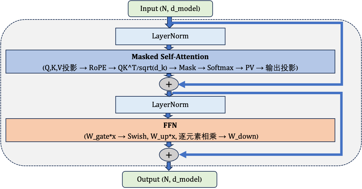
Note the Masked Self-Attention: in a Decoder, each token may only see itself and earlier tokens; it cannot peek ahead. That is done by adding an upper-triangular mask to the attention score matrix: future positions get , and after softmax their weights become 0.
7.2 Dimension tracking
Track tensor shapes with LLaMA-2-7B’s config:
- hidden_dim () = 4096
- num_heads () = 32
- head_dim () = 4096 / 32 = 128
- ffn_intermediate_dim = 11008 (SwiGLU intermediate width)
- sequence length = 2048 (example)
- batch_size = 1 (simplified; omit the batch dim)
Input:                     (2048, 4096)

── LayerNorm ──
LayerNorm(Input):          (2048, 4096)       # shape unchanged

── Masked Self-Attention ──
Q = LN(x) * W_Q:          (2048, 4096) x (4096, 4096) = (2048, 4096)
  → reshape:              (2048, 32, 128)     # 32 heads, 128 dims each
K = LN(x) * W_K:          (2048, 4096) → (2048, 32, 128)
V = LN(x) * W_V:          (2048, 4096) → (2048, 32, 128)

Apply RoPE to Q, K:       shape unchanged; rotate each head's 128 dims

# Each head computes Attention independently (head_i as example):
S_i = Q_i * K_i^T:        (2048, 128) x (128, 2048) = (2048, 2048)
S_i = S_i / sqrt(128):    (2048, 2048)         # scale
S_i = S_i + mask:         (2048, 2048)         # causal mask
A_i = softmax(S_i):       (2048, 2048)         # each row sums to 1
O_i = A_i * V_i:          (2048, 2048) x (2048, 128) = (2048, 128)

# Concatenate 32 head outputs:
O = concat(O_1,...,O_32):  (2048, 4096)
Output = O * W_O:          (2048, 4096) x (4096, 4096) = (2048, 4096)

── Residual Add ──
h = Input + Output:        (2048, 4096)

── LayerNorm ──
LayerNorm(h):              (2048, 4096)

── FFN (SwiGLU) ──
gate = LN(h) * W_gate:    (2048, 4096) x (4096, 11008) = (2048, 11008)
up   = LN(h) * W_up:      (2048, 4096) x (4096, 11008) = (2048, 11008)
mid  = Swish(gate) * up:   (2048, 11008)       # element-wise multiply
down = mid * W_down:       (2048, 11008) x (11008, 4096) = (2048, 4096)

── Residual Add ──
Output = h + down:         (2048, 4096)
From start to finish the data shape stays . That property matters: Blocks stack like bricks; one Block’s output is the next Block’s input with fully compatible dimensions.
7.3 Hand-counting parameters: where LLaMA-2-7B’s parameters go
Given config:
- num_heads = 32, head_dim = 128
- ffn_intermediate_dim = 11008
- num_layers = 32
- vocab_size = 32000
Parameters in one Decoder Block:
| Module | Parameter matrices | Parameter count |
|---|---|---|
| Attention | 16,777,216 | |
| Attention | 16,777,216 | |
| Attention | 16,777,216 | |
| Attention | 16,777,216 | |
| FFN | 45,088,768 | |
| FFN | 45,088,768 | |
| FFN | 45,088,768 | |
| LayerNorm x 2 | 4096 each | 16,384 |
| Per-Block total | ~201M |
Parameters for the full model:
| Component | How it is computed | Parameter count |
|---|---|---|
| Token Embedding | vocab_size = | ~131M |
| 32 Decoder Blocks | ~6,432M | |
| Final LayerNorm | ~8K | |
| Output head (LM Head) | vocab_size = | ~131M |
| Total | ~6,738M ≈ 6.7B |
Note: LLaMA-2 keeps separate Token Embedding and LM Head weights (no weight tying), so 6.7B already includes two copies of 131M. If you share weights like GPT-2, you subtract one 131M and land near 6.6B. The official “7B” label is a rounded approximation.
From the parameter split:
- FFN is about 67% (135M / 201M per layer)
- Attention is about 33% (67M / 201M per layer)
- Embedding is a small share (131M / 6738M ≈ 2%)
AI Infra note: Being able to hand-count these parameters is the basis of memory planning. Under mixed precision + Adam training (ZeRO paper accounting, 16Ψ Bytes/param total):
- FP16 weights: 6.7B × 2 Bytes = ~13.4 GB
- FP16 gradients: 6.7B × 2 Bytes = ~13.4 GB
- Adam FP32 state (FP32 master weights + first moment m + second moment v, 12 Bytes/param): 6.7B × 12 Bytes = ~80.4 GB
- Total: 6.7B × 16 Bytes ≈ ~107 GB
That is why a single 80GB A100 cannot train a 7B model: static memory alone already overflows, and with Activation storage you almost always need ZeRO (sharding optimizer state / gradients / parameters) to finish training.
8. From Transformer to LLM: autoregressive generation
So far we have the Transformer’s internal structure. How does a trained model actually generate text? This section covers how Transformer works at inference time, which ties directly into inference optimization.
8.1 Autoregressive generation: one token at a time
Large language model (LLM) text generation is autoregressive: at each step, given all tokens so far, predict the most likely next token.
User input: "The core of AI"
Step 1: "The core of AI"  → model predicts next token → " is"
Step 2: "The core of AI is" → model predicts next token → " Transformer"
Step 3: "The core of AI is Transformer" → model predicts next token → " architecture"
...
until <EOS> or max length
Each “prediction” is a full forward pass of every current token through the Transformer. The last layer’s output goes through the LM Head (a linear layer) to a vocab-sized vector, then softmax yields a distribution over tokens, and you sample the next one.
Generating one token at a time has a serious efficiency problem: every new token re-computes K and V in Attention for all history tokens. If the sequence length is , generating tokens costs in total, because each step’s Attention is and .
That leads to the central optimization in LLM inference: the KV Cache.
8.2 Prefill and Decode
LLM inference actually has two phases with very different characteristics:
Prefill
Process the entire user prompt. All input tokens can be computed in parallel; one forward pass produces K and V for every token and caches them.
Input: "Please explain what attention is" (assume 10 tokens)
→ 10 tokens enter the Transformer in parallel
→ each layer computes Q, K, V and caches K, V
→ one forward pass completes
→ emit the first generated token
Prefill’s matmuls have a large batch dimension ( tokens together). It is a classic Compute Bound workload. Its latency determines TTFT (Time To First Token).
Decode
Generate output tokens one by one. Each step has only one new token’s Q attending to all historical K; the new token’s K and V are appended to the cache.
Step 1: 1 new token's Q × 10 historical K → Attention → emit "at"
Step 2: 1 new token's Q × 11 historical K → Attention → emit "ten"
...
Decode has only one token of compute per step. Matmul collapses to matrix-vector multiply; the GPU’s compute sits mostly idle, and most time is spent moving KV Cache data from HBM. That is a classic Memory Bound workload. Its latency determines TPOT (Time Per Output Token).
AI Infra note: Prefill is Compute Bound and Decode is Memory Bound. The two phases have opposite bottlenecks, which led to Prefill/Decode disaggregation system designs (DistServe, Splitwise, and others) that place the two request types on different GPU pools and optimize each separately.
8.3 Where the KV Cache comes from
The KV Cache idea is simple: K and V that were already computed do not need to be computed again.
During Decode, every new token needs that token’s Q dotted with every historical token’s K. Without a cache, every step re-runs QKV projection over all history tokens. Those projections were already done in earlier steps; recomputing them is pure waste.
The KV Cache stores each layer’s K and V from each step in GPU memory. At Decode time the new token only computes its own Q, K, V; the new K and V are appended to the cache; Attention uses the full cached K and V.
Without KV Cache (recompute all KV every step): Step recomputes QKV for all tokens, cost ; total .
With KV Cache (only the new token’s KV): Step computes QKV for 1 new token (), and Attention dots 1 Q with cached K (); total .
KV Cache drops total QKV projection cost from to , at the price of extra memory for K and V of every layer and every token.
KV Cache memory cost:
For LLaMA-2-7B:
- Per token you cache: 2 (K and V) × 32 (layers) × 32 (heads) × 128 (head_dim) = 262,144 elements
- At FP16, 2 Bytes per element → KV Cache per token = 512 KB
- Sequence length 4096 → KV Cache per request = 4096 × 512 KB = 2 GB
- batch_size = 16 → total KV Cache = 16 × 2 GB = 32 GB
32 GB of KV Cache already takes 40% of an 80 GB GPU, plus 13.4 GB of model weights, so little room remains for other overhead. That is why KV Cache management is a central topic in inference optimization. Techniques like PagedAttention (virtual-memory paging), KV Cache quantization (store at lower precision), and GQA (fewer KV heads) all attack this “memory assassin”.
AI Infra note: KV Cache is the resource that needs the most careful management in inference deployment. The engineering problems it creates include memory fragmentation (different requests have different sequence lengths, so different KV Cache sizes), dynamic growth (KV Cache keeps growing during Decode), and multi-request sharing (Prefix Cache when system prompts match). Core innovations in engines like vLLM’s PagedAttention and SGLang’s RadixAttention are, at root, about managing KV Cache more efficiently.
📝 Summary
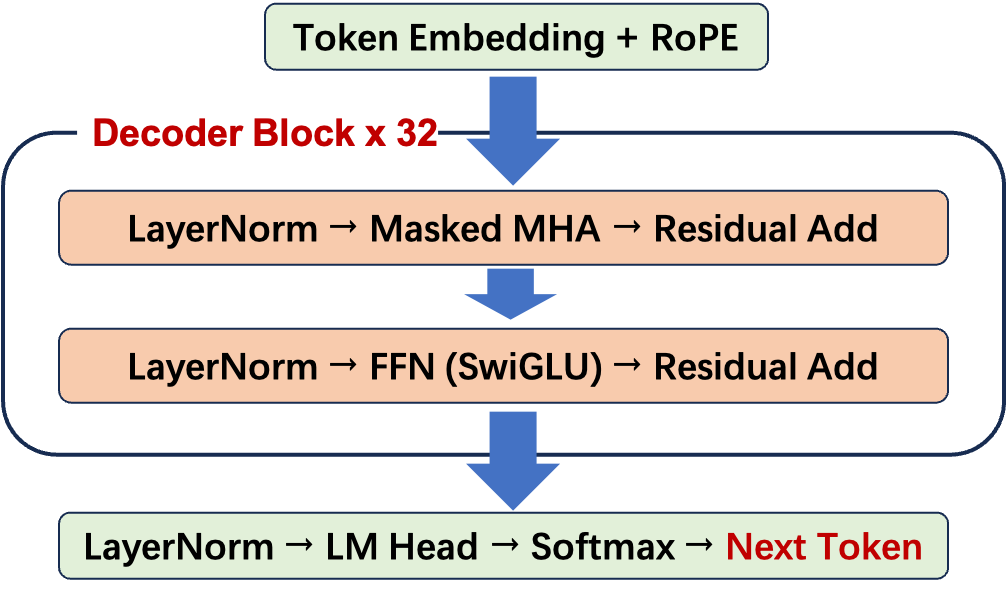
Here is the full Transformer Decoder Block structure again, plus how each module ties into later AI Infra topics:
| Module | Core compute | Later AI Infra links |
|---|---|---|
| Self-Attention | , Softmax, PV | FlashAttention (CUDA), KV Cache (inference), tensor parallel along heads |
| Multi-Head | Independent heads then concat | Tensor parallel (TP) shard point, GQA/MQA (inference) |
| FFN (SwiGLU) | Three large matmuls | Parameter bulk, another TP shard point, MoE expert parallel |
| LayerNorm | Mean/variance normalize | Kernel fusion, RMSNorm simplification |
| Residual | Element-wise add | Fuse with LayerNorm, gradient-flow analysis |
| Positional encoding (RoPE) | Rotate Q/K | Fuse into Attention kernel, long-context extension |
| KV Cache | Cache historical K, V | PagedAttention, KV quantization, Prefix Cache |
| Autoregressive generation | Prefill + Decode | Prefill/Decode disaggregation, Speculative Decoding |
Learning Transformer architecture is not the end goal; it is the starting point. Once you know what the optimization target looks like, later AI Infra techniques stop floating in the air. FlashAttention attacks the memory issue in section 3.3, tensor parallelism shards the multi-head layout in 3.4 and the FFN matrices in 4.2, and KV Cache management deals with the memory cost in 8.3.
🎯 Self-check list
After reading this article, check whether you really understand Transformer architecture:
- Without notes, draw a full Decoder Block on a whiteboard (Masked Self-Attention → Add & Norm → FFN → Add & Norm) and label input/output dimensions at each step
- Explain the differences among Encoder-Decoder, Encoder-only, and Decoder-only, and why large models mostly use Decoder-only
- Explain what Q, K, and V each mean, and the physical meaning of every element in the attention score matrix
- Write the full Attention formula from memory, and explain why we divide by
- Derive Self-Attention’s complexity, and explain how that led to FlashAttention
- Explain why Multi-Head Attention fits tensor-parallel sharding, and how GQA improves on MHA for KV Cache
- Hand-count LLaMA-2-7B’s total parameters (within 20%), and state the FFN vs Attention parameter ratio
- Explain how Prefill and Decode differ in compute character (Compute Bound vs Memory Bound), and where the KV Cache comes from
- Estimate KV Cache memory for a given config (e.g. 7B model, sequence length 4096, batch_size=16 ≈ 32 GB)
📚 References
Papers
- Attention Is All You Need (Vaswani et al., 2017): https://arxiv.org/abs/1706.03762 — original Transformer paper; required reading
- RoFormer: Enhanced Transformer with Rotary Position Embedding (Su et al., 2021): https://arxiv.org/abs/2104.09864 — RoPE rotary positional encoding
- GLU Variants Improve Transformer (Shazeer, 2020): https://arxiv.org/abs/2002.05202 — SwiGLU and other gated activations
- LLaMA: Open and Efficient Foundation Language Models (Touvron et al., 2023): https://arxiv.org/abs/2302.13971 — LLaMA model architecture
- LLaMA 2: Open Foundation and Fine-Tuned Chat Models (Touvron et al., 2023): https://arxiv.org/abs/2307.09288 — LLaMA-2 technical report
- FlashAttention: Fast and Memory-Efficient Exact Attention with IO-Awareness (Dao et al., 2022): https://arxiv.org/abs/2205.14135 — memory-aware Attention optimization
- GQA: Training Generalized Multi-Query Transformer Models from Multi-Head Checkpoints (Ainslie et al., 2023): https://arxiv.org/abs/2305.13245 — Grouped-Query Attention
Tutorials and blogs
- The Illustrated Transformer (Jay Alammar): https://jalammar.github.io/illustrated-transformer/ — illustrated Transformer intro
- Andrej Karpathy: Let’s build GPT from scratch: https://www.youtube.com/watch?v=kCc8FmEb1nY — write GPT from scratch; code-level view of every module
- 3Blue1Brown: But what is a GPT: https://www.youtube.com/watch?v=wjZofJX0v4M — intuitive view of Transformer
- The Annotated Transformer (Harvard NLP): https://nlp.seas.harvard.edu/annotated-transformer/ — paper line-by-line with PyTorch