6.1 FlashAttention V1 in detail

This article digs into the core ideas and implementation details of FlashAttention V1: how Tiling + Online Softmax cut Attention’s extra GPU memory from $O(N^2)$ to $O(N)$, slash HBM traffic, and speed things up with no accuracy loss.

📑 Contents

• 1. Performance bottlenecks of standard Attention
• 2. Core idea of FlashAttention
• 3. Online Softmax algorithm
• 4. Tiling strategy
• 5. Full forward pass
• 6. Backward pass and recomputation
• 7. IO complexity analysis
• 8. Implementation notes and code examples
• Summary
• Self-check list
• References

---

1. Performance bottlenecks of standard Attention

1.1 Standard Attention compute flow

Scaled Dot-Product Attention runs as:

$$S = QK^\top / \sqrt{d}$$ $$P = \text{softmax}(S)$$ $$O = PV$$

where $Q, K, V \in \mathbb{R}^{N \times d}$, $N$ is sequence length, and $d$ is head dimension.

1.2 Memory bottleneck analysis

The key problem in the standard implementation is that intermediate matrices $S$ and $P$ are $N \times N$:

At sequence length $N = 4096$, $d = 128$, a single head’s $S$ alone needs $4096 \times 4096 \times 2 = 32$ MB (FP16). With multiple heads and batches, memory cost is huge.

1.3 Insufficient arithmetic intensity

Arithmetic Intensity of standard Attention is:

$$\text{AI} = \frac{O(N^2 d)}{O(N^2 + Nd)} \approx O(d)$$

Since $d$ is usually only 64 or 128, arithmetic intensity is low — the bottleneck is memory bandwidth, not compute. A lot of time goes to data movement while GPU compute units starve.

💡 Tip: like a chef who cooks fast but waits forever for ingredients from the warehouse — the core bottleneck of standard Attention is data movement between HBM and SRAM.

---

2. Core idea of FlashAttention

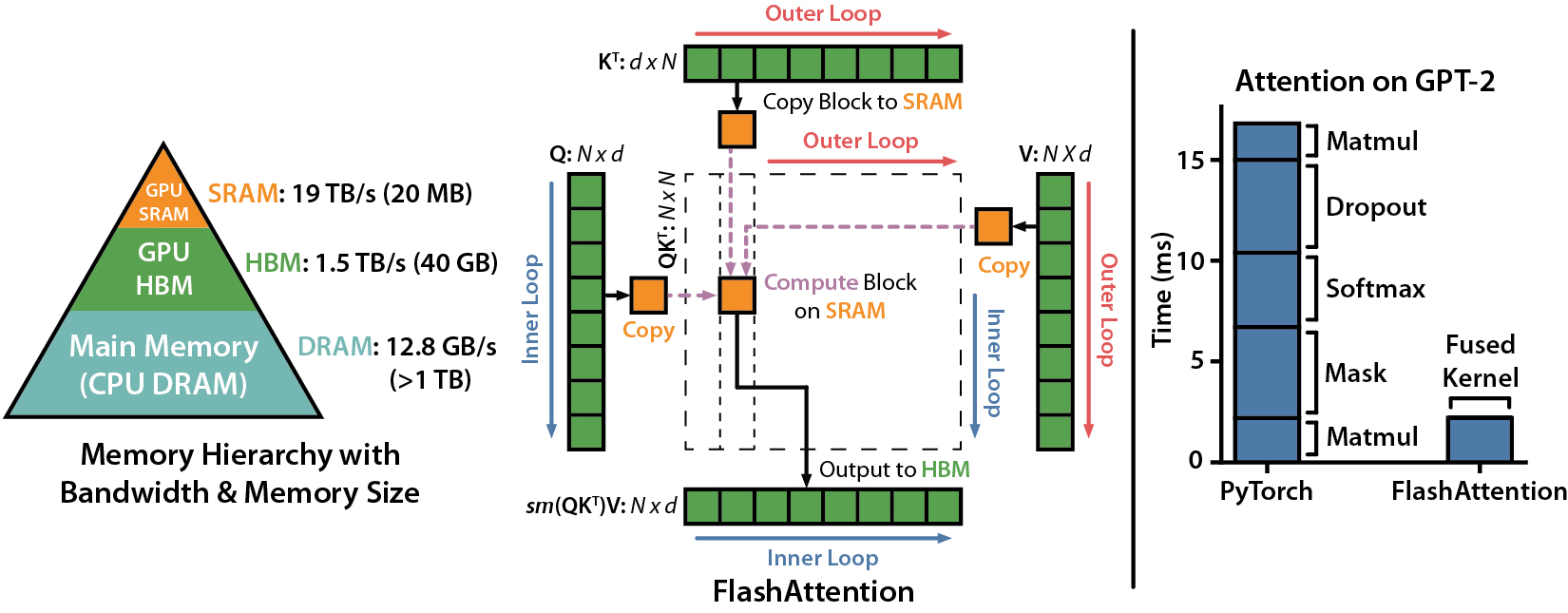
2.1 IO-Awareness: focus on data movement

FlashAttention’s core insight: on modern GPUs, Attention is Memory-Bound; the win is fewer HBM accesses, not fewer FLOPs.

Traditional optimization chases fewer FLOPs (e.g. sparse Attention). FlashAttention takes another path — clever tiling keeps data in SRAM (Shared Memory) as much as possible and avoids landing intermediate results in HBM.

2.2 Two key techniques

FlashAttention V1 combines two techniques:

1. Tiling: cut Q, K, V into small tiles; load one tile at a time into SRAM to compute
2. Online Softmax: without knowing the global max, correct Softmax results as new tiles arrive

📌 Key point: both are required — Tiling solves “how not to materialize the full $N \times N$ matrix”; Online Softmax solves “Softmax needs global info when computing in tiles”.

2.3 Intuition

Imagine ranking every student by percentile from the whole class’s scores. The usual way collects every score (all on the blackboard) then computes. FlashAttention is more like: each time a group of scores arrives, immediately update running stats (max, sum) and correct previous results — the final answer matches collecting everything first.

---

3. Online Softmax algorithm

3.1 Three passes of standard Softmax

For numerical stability, standard (safe) Softmax needs three passes over $x \in \mathbb{R}^N$:

Pass 1: global max for numerical stability

$$m = \max_{i=1}^{N} x_{i}$$

Pass 2: normalization denominator (exp-sum)

$$\ell = \sum_{j=1}^{N} e^{x_j - m}$$

Pass 3: normalized output per element

$$\text{softmax}(x_i) = \frac{e^{x_i - m}}{\ell}$$

Passes 2 and 3 both need the global max $m$ from pass 1; pass 3 also needs $\ell$ from pass 2. You must finish a full scan before the next — which conflicts with tiling.

📖 Further reading: Online Softmax (NVIDIA, 2018) merges the three passes into two — maintain $m$ and $\ell$ while scanning; FlashAttention further fuses “multiply by $V$ for the output” into that flow.

3.2 Online Softmax recurrence

The key innovation: maintain correctable local stats and update them as new data tiles arrive.

Suppose the first $j-1$ tiles are done, with local max $m^{(j-1)}$ and local exp-sum $l^{(j-1)}$. When tile $j$, $x^{(j)}$, arrives:

Step 1: update max

$$m^{(j)} = \max(m^{(j-1)}, \max(x^{(j)}))$$

Step 2: correct and update exp-sum

$$l^{(j)} = l^{(j-1)} \cdot e^{m^{(j-1)} - m^{(j)}} + \sum_{i} e^{x^{(j)}_i - m^{(j)}}$$

Step 3: correct existing output

$$O^{(j)} = O^{(j-1)} \cdot \frac{l^{(j-1)} \cdot e^{m^{(j-1)} - m^{(j)}}}{l^{(j)}} + \frac{\sum_i e^{x^{(j)}_i - m^{(j)}} \cdot V^{(j)}_i}{l^{(j)}}$$

3.3 Correctness

Mathematical correctness comes from a simple identity:

$$e^{x_i - m_{\text{new}}} = e^{x_i - m_{\text{old}}} \cdot e^{m_{\text{old}} - m_{\text{new}}}$$

Whenever the global max updates, every previous exp term is fixed by multiplying $e^{m_{\text{old}} - m_{\text{new}}}$. The operation is exact — no approximation.

⚠️ Note: Online Softmax is mathematically equivalent to standard Softmax (aside from tiny rounding differences from floating-point order). It is not an approximate algorithm.

---

4. Tiling strategy

4.1 Tiling scheme

Split $Q$, $K$, $V$ along the sequence dimension into tiles of size $B_r$ (Q tile size) and $B_c$ (K/V tile size):

• $Q$ into $T_r = \lceil N / B_r \rceil$ tiles
• $K, V$ into $T_c = \lceil N / B_c \rceil$ tiles

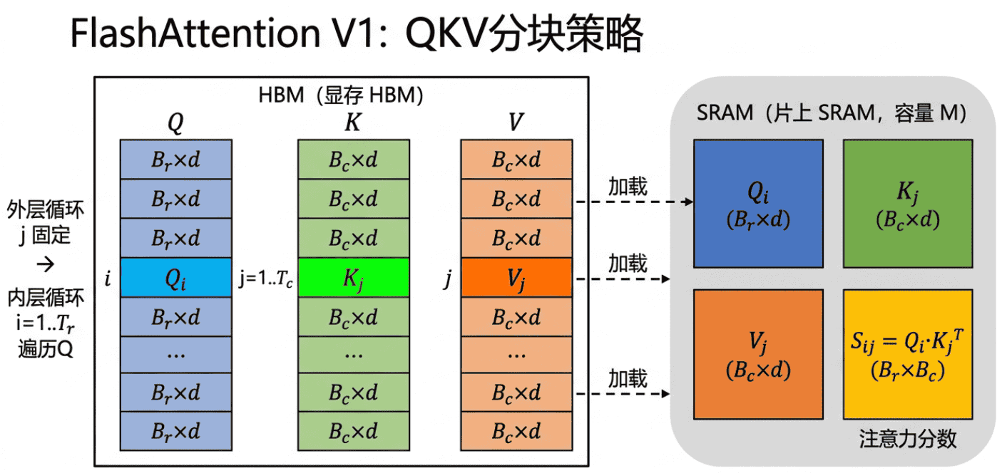
Tile size depends on SRAM capacity $M$ (in elements; think M = SRAM_bytes / sizeof(dtype)) and head dimension $d$ (feature dim per token, e.g. $d = 128$ in LLaMA-7B):

$$B_c = \left\lceil \frac{M}{4d} \right\rceil, \quad B_r = \min\left(\left\lceil \frac{M}{4d} \right\rceil, d\right)$$

Why $\dfrac{M}{4d}$?

Computing one tile, SRAM must hold $Q_i, K_j, V_j, O_i$ — four tensors roughly $B \times d$ (see §4.2), about $4 B d$ elements. Require $4 B d \le M$, so each tile holds at most $\dfrac{M}{4d}$ rows. Relatively small $S_{ij}$ ($B_r \times B_c$) and stats $m_i, l_i$ ($2B_r$) are ignored because when $B \ll d$ they do not dominate SRAM.

Why also $\min$ $B_r$ with $d$?

Online Softmax’s correction $e^{m^{(j-1)} - m^{(j)}}$ is a per-row scalar. The original paper constrains $B_r \le d$ to simplify analysis and avoid complicated stats management when rows greatly exceed the column dim; V2 relaxes this.

4.2 SRAM layout

During compute, SRAM must hold:

Total SRAM is about $(2B_r + 2B_c) \times d + B_r \times B_c + 2B_r$; the dominant term is $(2B_r + 2B_c) \times d$, which is why the tile-size formula has $4d$ in the denominator — stay under Shared Memory capacity $M$.

4.3 Outer and inner loops

FlashAttention V1 uses outer loop over K/V tiles, inner loop over Q tiles:

outer: for j = 1 to T_c (iterate K/V tiles)
    load K_j, V_j from HBM into SRAM
    inner: for i = 1 to T_r (iterate Q tiles)
        load Q_i, O_i, m_i, l_i from HBM into SRAM
        compute local scores S_ij = Q_i * K_j^T
        update stats and output
        write updated O_i, m_i, l_i back to HBM

💡 Tip: outer over K/V means each K/V tile loads from HBM once, while Q and O load many times. That is a V1 weakness (V2 flips to outer over Q).

---

5. Full forward pass

5.1 Step-by-step derivation

For the $i$-th Q tile and $j$-th K/V tile:

Step 1: local attention scores

$$S_{ij} = Q_i K_j^\top / \sqrt{d} \in \mathbb{R}^{B_r \times B_c}$$

Step 2: current tile row-max

$$\tilde{m}_{ij} = \text{rowmax}(S_{ij}) \in \mathbb{R}^{B_r}$$

Step 3: update global row-max

$$m_i^{\text{new}} = \max(m_i, \tilde{m}_{ij})$$

Step 4: correction factor and update exp-sum

$$\alpha = e^{m_i - m_i^{\text{new}}}$$ $$l_i^{\text{new}} = \alpha \cdot l_i + \text{rowsum}\left(e^{S_{ij} - m_i^{\text{new}}}\right)$$

$\alpha$ rescales the old exp-sum $l_i$ (under old max $m_i$) onto the new max $m_i^{\text{new}}$.

Step 5: update output

$$O_i^{\text{new}} = \frac{\alpha \cdot l_i}{l_i^{\text{new}}} \cdot O_i + \frac{1}{l_i^{\text{new}}} \cdot e^{S_{ij} - m_i^{\text{new}}} \cdot V_j$$

5.2 Algorithm pseudocode

# FlashAttention V1 forward pseudocode
def flash_attention_forward(Q, K, V, B_r, B_c):
    N, d = Q.shape
    O = zeros(N, d)
    m = full(N, -inf)  # row max
    l = zeros(N)        # row exp-sum

    # Outer loop: iterate K/V tiles
    for j in range(0, N, B_c):
        K_j = K[j:j+B_c]  # load from HBM
        V_j = V[j:j+B_c]  # load from HBM

        # Inner loop: iterate Q tiles
        for i in range(0, N, B_r):
            Q_i = Q[i:i+B_r]          # load from HBM
            O_i = O[i:i+B_r]          # load from HBM
            m_i = m[i:i+B_r]          # load from HBM
            l_i = l[i:i+B_r]          # load from HBM

            # Local attention scores
            S_ij = Q_i @ K_j.T / sqrt(d)  # [B_r, B_c]

            # Update stats
            m_new = max(m_i, rowmax(S_ij))
            l_new = l_i * exp(m_i - m_new) + rowsum(exp(S_ij - m_new))

            # Update output
            O_new = O_i * (l_i * exp(m_i - m_new) / l_new).unsqueeze(1)
            O_new += (exp(S_ij - m_new) / l_new.unsqueeze(1)) @ V_j

            # Write back to HBM
            O[i:i+B_r] = O_new
            m[i:i+B_r] = m_new
            l[i:i+B_r] = l_new

    return O

5.3 Numerical stability

The whole path stays stable by subtracting the max:

• Every exp input is shifted by the current known max, so $e^x$ has $x \leq 0$
• Correction $e^{m_{\text{old}} - m_{\text{new}}}$ also has $m_{\text{old}} \leq m_{\text{new}}$, hence $\leq 1$

No overflow in the full computation.

---

6. Backward pass and recomputation

6.1 Backward challenge

Standard Attention backward needs intermediate $S$ and $P$ ($N \times N$) for gradients. $S = QK^\top / \sqrt{d}$ is pre-softmax logits; $P = \text{softmax}(S)$ is post-softmax attention weights; output $O = PV$:

$$dV = P^\top dO$$ $$dP = dO \cdot V^\top$$ $$dS = P \odot \left(dP - \text{rowsum}(dP \odot P) \cdot \mathbf{1}^\top\right)$$

FlashAttention uses the identity $\text{rowsum}(dP \odot P) = \text{rowsum}(dO \odot O)$ (written $D_i$) to avoid building the full $dP$ matrix.

Saving those intermediates would waste the memory the forward pass saved.

6.2 Recomputation strategy

FlashAttention V1 does not save $S$ and $P$; it recomputes them in backward:

• Forward only saves: $Q, K, V, O, m, l$ (inputs, output, stats)
• Backward: with saved $m$ and $l$, reload $Q_i, K_j$ to form $S_{ij}$, then recover $P_{ij}$

$$P_{ij} = \text{diag}(l_i)^{-1} \cdot e^{S_{ij} - m_i}$$

6.3 Cost of recomputation

Recomputation adds FLOPs (about one extra forward matmul), but HBM traffic drops:

Because Attention is Memory-Bound, the extra compute is “hidden” by fewer HBM accesses — wall-clock time is often shorter.

---

7. IO complexity analysis

7.1 Standard Attention IO complexity

$$\text{HBM 访问量} = O(Nd + N^2) = O(N^2)$$

$Nd$ comes from reading/writing $Q, K, V, O$ ($N \times d$); $N^2$ from intermediate $S$ and $P$ (each $N \times N$). When $N \gg d$, $N^2$ dominates → $O(N^2)$.

7.2 FlashAttention IO complexity

FlashAttention HBM traffic:

$$\text{HBM 访问量} = O\left(\frac{N^2 d^2}{M}\right)$$

Breakdown:

• From §4.1, $B_c = O(M/d)$, so $T_c = N / B_c = O(Nd/M)$ outer iterations
• Each outer pass sweeps full $Q$ and $O$ ($O(Nd)$ elements), so $Q$ and $O$ traffic is $T_c \cdot Nd = O(N^2 d^2 / M)$
• $K, V$ are each read once: $O(Nd)$, negligible next to the above

Total $O(N^2 d^2 / M)$. Intuition: larger SRAM ($M$) → larger tiles → fewer outer loops → less repeated $Q/O$ traffic.

$M$ is SRAM size in elements. Since $d^2 < M$ (typical $d = 128$, $M$ ≈ $192 \text{KB} / 2 = 98304$ FP16 elements, $d^2 = 16384$), this is much smaller than $O(N^2)$.

7.3 Lower-bound proof

The paper also shows any exact Attention algorithm needs at least $\Omega(N^2 d^2 / M)$ HBM accesses — FlashAttention’s IO complexity is asymptotically optimal.

7.4 Practical speedup

Typical A100 comparison:

---

8. Implementation notes and code examples

8.1 Tensor shapes end to end

Inputs $Q, K, V$ are 4-D; the first two dims are batch and head (passed through as “batch”); the last two do the matmuls:

Q: [B, H, N, D]
K: [B, H, N, D]   →  K^T (transpose last two dims): [B, H, D, N]
V: [B, H, N, D]

Step 1  Attention scores:
  S = Q @ K^T / sqrt(D)
    = [B, H, N, D] @ [B, H, D, N]
    = [B, H, N, N]

Step 2  Softmax (along last N, row-wise):
  P = softmax(S, dim=-1)
    shape: [B, H, N, N]

Step 3  Output:
  O = P @ V
    = [B, H, N, N] @ [B, H, N, D]
    = [B, H, N, D]   (same shape as Q)

Auxiliary tensors (FlashAttention-specific):

• M: [B, H, N] — per-row max (numerical stability + Online Softmax correction)
• L: [B, H, N] — per-row exp-sum (softmax denominator)

8.2 Kernel design notes

📌 On parallel partitioning (grid and block design):

• grid (program granularity) = (B, H): each program owns full attention for one (batch, head) slice; programs are independent, no communication.
• Threads inside a block: within a program, Triton splits tl.dot, tl.max, tl.sum, etc. across warps of a thread block. Tile size is set by BLOCK_M (Q rows $B_r$), BLOCK_N (K/V rows $B_c$), BLOCK_D (vectorized width on D).
• Serial inside a program: outer loop over K/V tiles, inner over Q tiles

Different Q tiles share stats $m_i, l_i$ and accumulated $O_i$ across outer iterations; one program’s registers cannot hold m/l/O for “all Q tiles”, so HBM auxiliaries M, L persist across iterations (the root cause of V1’s extra IO — V2 swaps loop order, puts Q on the grid, and keeps m/l/O in registers the whole time, removing that HBM traffic).

⚠️ V1’s natural parallelism bottleneck: grid size $B \times H$ in inference is often only tens (e.g. batch=1, heads=32 → 32 programs), while modern GPUs have 80–140 SMs (A100=108, H100=132), so SM utilization is ~30%. That is V1’s main weakness and the reason V2 had to appear.

1. Thread Block mapping: in V1 each Thread Block owns one outer K/V tile (one $j$) and walks all Q tiles
2. Shared Memory: pre-allocate SRAM for $K_j$, $V_j$ (resident in the outer loop) plus $Q_i$, $S_{ij}$
3. Registers: keep stats $m_i$, $l_i$ and accumulated $O_i$ in registers when possible
4. Loop structure: outer loads K/V tiles; inner does GEMM and Softmax updates

8.3 Simplified Triton implementation

import math
import torch
import triton
import triton.language as tl

@triton.jit
def flash_attn_v1_kernel(
    Q, K, V, O,    # [B, H, N, D]
    M, L,          # row max and row exp-sum
    stride_qb, stride_qh, stride_qn, stride_qd,
    stride_kb, stride_kh, stride_kn, stride_kd,
    stride_vb, stride_vh, stride_vn, stride_vd,
    stride_ob, stride_oh, stride_on, stride_od,
    stride_mb, stride_mh,
    N,
    D: tl.constexpr,        # head dimension (feature length per token); used in scale = 1/sqrt(D)
    BLOCK_M: tl.constexpr,  # Q tile rows B_r
    BLOCK_N: tl.constexpr,  # K/V tile rows B_c
    BLOCK_D: tl.constexpr,  # load/compute width on head dim; when D is a power of 2, BLOCK_D==D; else BLOCK_D > D and excess positions are masked
):
    # ========== V1 parallel partition: grid = (batch, head) ==========
    # Each program serially sweeps all K/V and Q tiles for one (batch, head)
    batch_id = tl.program_id(0)
    head_id = tl.program_id(1)

    # Base offsets of current (batch, head) on each tensor
    qkvo_bh_q = batch_id * stride_qb + head_id * stride_qh
    qkvo_bh_k = batch_id * stride_kb + head_id * stride_kh
    qkvo_bh_v = batch_id * stride_vb + head_id * stride_vh
    qkvo_bh_o = batch_id * stride_ob + head_id * stride_oh
    ml_bh = batch_id * stride_mb + head_id * stride_mh

    d_range = tl.arange(0, BLOCK_D)
    scale = 1.0 / math.sqrt(D)

    # ============ Outer loop: iterate K/V tiles (V1 key design) ============
    for kv_start in range(0, N, BLOCK_N):
        kv_range = kv_start + tl.arange(0, BLOCK_N)
        kv_mask = kv_range < N

        # Load K_j, V_j once; stay in registers/SRAM; reused by all Q tiles
        k = tl.load(K + qkvo_bh_k + kv_range[:, None] * stride_kn + d_range[None, :] * stride_kd,
                    mask=kv_mask[:, None] & (d_range[None, :] < D), other=0.0)
        v = tl.load(V + qkvo_bh_v + kv_range[:, None] * stride_vn + d_range[None, :] * stride_vd,
                    mask=kv_mask[:, None] & (d_range[None, :] < D), other=0.0)

        # ============ Inner loop: iterate Q tiles ============
        for q_start in range(0, N, BLOCK_M):
            q_range = q_start + tl.arange(0, BLOCK_M)
            q_mask = q_range < N

            # Load Q_i, O_i, m_i, l_i — in V1 every outer iter reloads from HBM
            q = tl.load(Q + qkvo_bh_q + q_range[:, None] * stride_qn + d_range[None, :] * stride_qd,
                        mask=q_mask[:, None] & (d_range[None, :] < D), other=0.0)
            o_i = tl.load(O + qkvo_bh_o + q_range[:, None] * stride_on + d_range[None, :] * stride_od,
                          mask=q_mask[:, None] & (d_range[None, :] < D), other=0.0).to(tl.float32)
            m_i = tl.load(M + ml_bh + q_range, mask=q_mask, other=float('-inf'))
            l_i = tl.load(L + ml_bh + q_range, mask=q_mask, other=0.0)

            # S_ij = Q_i @ K_j^T / sqrt(d)
            s = tl.dot(q, tl.trans(k)) * scale
            # Mask out-of-range K/V columns so fake 0s do not pollute the softmax denominator
            s = tl.where(kv_mask[None, :], s, float('-inf'))

            # Online Softmax update
            m_new = tl.maximum(m_i, tl.max(s, axis=1))
            alpha = tl.exp(m_i - m_new)
            p = tl.exp(s - m_new[:, None])
            l_new = alpha * l_i + tl.sum(p, axis=1)

            # Output correction + accumulate (matches §5.1 Step 5)
            o_new = o_i * (alpha * l_i / l_new)[:, None] \
                    + tl.dot(p.to(v.dtype), v) / l_new[:, None]

            # Write updated O_i, m_i, l_i back to HBM for the next outer iter
            tl.store(O + qkvo_bh_o + q_range[:, None] * stride_on + d_range[None, :] * stride_od,
                     o_new.to(O.dtype.element_ty),
                     mask=q_mask[:, None] & (d_range[None, :] < D))
            tl.store(M + ml_bh + q_range, m_new, mask=q_mask)
            tl.store(L + ml_bh + q_range, l_new, mask=q_mask)


def flash_attn_v1(Q, K, V, BLOCK_M=64, BLOCK_N=64):
    # Q, K, V: [B, H, N, D]
    B, H, N, D = Q.shape
    O = torch.zeros_like(Q)
    M = torch.full((B, H, N), float('-inf'), device=Q.device, dtype=torch.float32)
    L = torch.zeros((B, H, N), device=Q.device, dtype=torch.float32)

    BLOCK_D = triton.next_power_of_2(D)
    grid = (B, H)  # V1 parallel: only on batch×head
    flash_attn_v1_kernel[grid](
        Q, K, V, O, M, L,
        Q.stride(0), Q.stride(1), Q.stride(2), Q.stride(3),
        K.stride(0), K.stride(1), K.stride(2), K.stride(3),
        V.stride(0), V.stride(1), V.stride(2), V.stride(3),
        O.stride(0), O.stride(1), O.stride(2), O.stride(3),
        M.stride(0), M.stride(1),
        N, D=D, BLOCK_M=BLOCK_M, BLOCK_N=BLOCK_N, BLOCK_D=BLOCK_D,
    )
    return O

📌 Code takeaways:

1. V1 parallel partition: grid is (batch, head), K/V outer, Q inner — each K/V tile loads from HBM once, but Q/O/m/l are read/written $T_c$ times
2. Auxiliary M, L: stats $m_i, l_i$ for Q must be shared across outer iters, so persist [B, H, N] tensors in HBM
3. K/V OOB mask (tl.where(kv_mask, s, -inf)) is critical for correctness; missing it pollutes the softmax denominator with fake zeros
4. Initial m, l are -inf and 0; with alpha = exp(-inf - m_new) = 0, the first iter naturally becomes a normal accumulate
5. V1 limit: (batch, head) is usually far below SM count (A100 has 108 SMs; batch×head in inference is often only tens), so SM utilization is low; V2 puts Q on the grid to fix that

---

📝 Summary

FlashAttention V1 rethinks Attention through IO-Awareness and proposes Tiling + Online Softmax:

1. No full $N \times N$ intermediate matrix — tiled streaming avoids $O(N^2)$ memory
2. Online Softmax stays exact — maintain and correct local stats for results equivalent to standard Softmax
3. Recompute instead of store — backward recomputes $S$ and $P$, trading a little compute for large memory savings
4. Asymptotically optimal IO — HBM traffic drops from $O(N^2)$ to $O(N^2 d^2 / M)$

---

🎯 Self-check list

• Explain why standard Attention is Memory-Bound rather than Compute-Bound
• Manually derive the Online Softmax recurrence update
• Show how tile sizes $B_r$, $B_c$ follow from SRAM capacity
• Describe what the outer and inner loops traverse in FlashAttention forward
• Explain why recomputation does not lengthen wall-clock time
• Derive FlashAttention HBM IO complexity $O(N^2 d^2 / M)$
• Implement a simplified FlashAttention forward Kernel in Triton or CUDA
• State the limitation of outer-looping K/V in FlashAttention V1

---

📚 References

• FlashAttention: Fast and Memory-Efficient Exact Attention with IO-Awareness
• Online Normalizer Calculation for Softmax
• FlashAttention official implementation - GitHub
• Tri Dao - FlashAttention paper notes
• NVIDIA CUDA C++ Programming Guide