CUDA programming quick start guide
A full walkthrough of the CUDA programming model, memory hierarchy, and common operator optimizations so you can implement and tune AI kernels efficiently
CUDA is the bridge between AI algorithms and GPU hardware. It turns high-level math into machine instructions the GPU can run as efficiently as possible. This guide starts from the programming model and memory hierarchy, covers Reduce / GEMM / Softmax as three classic operators, then FlashAttention-style Attention kernels and the Triton compiler. Together that is the CUDA foundation most AI Infra engineers need.
Table of contents
- 1. Environment setup
- 2. CUDA programming model
- 3. Memory model
- 4. Key concepts
- 5. First complete program: vector add
- 6. Common operators: implementation and optimization
- 7. Attention operators
- 8. AI compilers
- 9. Profiling tools
- 10. Advanced topics: putting the ideas together
- 11. Self-check list
- References
1. Environment setup
1.1 Hardware requirements
- NVIDIA GPU (Compute Capability >= 7.0, Volta and newer)
- At least 8GB of VRAM is recommended for operator development and debugging
What is Compute Capability? It is NVIDIA’s “capability version” for a GPU: which generation of PTX and which hardware features it supports. For example
sm_90is Hopper (H100),sm_100is Blackwell (B200). Knowing the number helps you read-arch=flags, and explains why the same binary may not run on an older card.
1.2 Software install
Install the CUDA Toolkit
# Ubuntu 22.04
wget https://developer.download.nvidia.com/compute/cuda/repos/ubuntu2204/x86_64/cuda-keyring_1.1-1_all.deb
sudo dpkg -i cuda-keyring_1.1-1_all.deb
sudo apt-get update
sudo apt-get install cuda-toolkit-12-3

# Set environment variables (add to ~/.bashrc or ~/.zshrc)
export PATH=/usr/local/cuda/bin:$PATH
export LD_LIBRARY_PATH=/usr/local/cuda/lib64:$LD_LIBRARY_PATH
Verify the install
nvcc --version          # CUDA compiler version
nvidia-smi              # GPU info and driver version
1.3 Compilation basics
CUDA sources use the .cu extension and compile with nvcc:
# Basic compile
nvcc hello.cu -o hello

# Target a GPU architecture (recommended)
nvcc -arch=sm_80 hello.cu -o hello    # A100
nvcc -arch=sm_90 hello.cu -o hello    # H100

# Print register and shared-memory usage (essential when tuning)
nvcc -Xptxas -v hello.cu -o hello
What happens after compile? The GPU compiler does not emit machine code in one step. It first produces PTX (a virtual ISA / IR), then JIT-compiles that to SASS (streaming assembler, the real instructions for that GPU generation) on the target GPU or when the driver installs. That is why one CUDA source can run later on a new physical GPU: as long as the new hardware supports that PTX version, the driver JITs matching SASS. Once you see that, flags like -arch=sm_90 make sense: they tell the compiler “generate code for H100-class hardware.”
2. CUDA programming model
2.1 Kernels
A kernel is a function that runs on the GPU. You declare it with __global__ and launch it with <<<gridDim, blockDim>>> to set the parallel shape:
// Declare a kernel
__global__ void myKernel(float* data, int n) {
    int idx = blockIdx.x * blockDim.x + threadIdx.x;
    if (idx < n) {
        data[idx] *= 2.0f;
    }
}

// Launch: 128 Blocks, 256 threads per Block
myKernel<<<128, 256>>>(data, n);
CUDA has three function qualifiers:
| Qualifier | Where it runs | Who can call it | Notes |
|---|---|---|---|
__global__ | GPU | CPU (or GPU) | Kernel; launches GPU parallel work |
__device__ | GPU | GPU | Device function; only callable from kernels or other device functions |
__host__ | CPU | CPU | Ordinary CPU function (default; can be omitted) |
You can combine __host__ and __device__ so the compiler emits both a CPU and a GPU version.
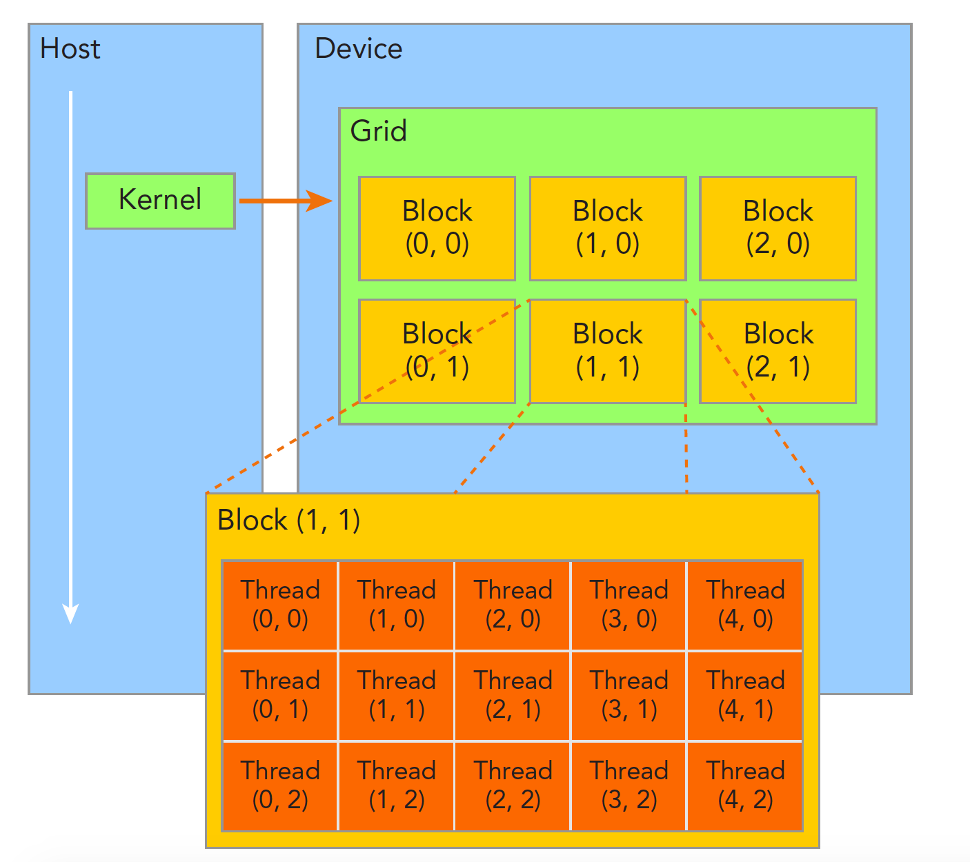
Terminology: Kernel, Grid, and CTA. At the PTX/SASS level, a thread block (Block) is a Cooperative Thread Array (CTA). Multiple Blocks form a Grid, the full set of threads created by one kernel launch. The Grid spans the whole GPU, so a kernel is the largest parallel unit you control as a programmer.
On hardware, a Block is scheduled onto one Streaming Multiprocessor (SM). How many SMs you have sets how many Blocks can run at once. Threads in the same Block can cooperate tightly (shared memory, barrier sync). Threads in different Blocks can only cooperate indirectly through global memory and atomics, and their order is undefined, so when you write a kernel you must not assume which Block runs first.
2.2 Grid / Block / Thread hierarchy
CUDA organizes threads in three levels. That hierarchy is the heart of parallel programming here. Think of it as “school / class / student”: the Grid is the school, a Block is a class, a Thread is a student. Each student does their own work, but classmates can talk through the “blackboard” (Shared Memory).
Dimensions and indices
Grid and Block both support 1D, 2D, and 3D. Global thread indices look like this:
// 1D (most common)
int idx = blockIdx.x * blockDim.x + threadIdx.x;

// 2D (common for matrix work)
int row = blockIdx.y * blockDim.y + threadIdx.y;
int col = blockIdx.x * blockDim.x + threadIdx.x;

// dim3 for 2D launch geometry
dim3 blockDim(16, 16);     // 16x16 = 256 threads per Block
dim3 gridDim(
    (width + 15) / 16,     // Blocks in x
    (height + 15) / 16     // Blocks in y
);
kernel<<<gridDim, blockDim>>>(data, width, height);
Hard limits
| Parameter | Limit |
|---|---|
| Threads per Block | up to 1024 |
| Blocks per Grid dimension | up to 2^31 - 1 (x), 65535 (y, z) |
| Active threads per SM | up to 2048 (64 Warps) |
| Active Blocks per SM | up to 32 |
Block size heuristics
- 256: good default for most cases (8 Warps)
- 128: memory-heavy work where you want more concurrent Blocks
- 512-1024: compute-heavy work; watch register and shared-memory pressure
- Always a multiple of 32: match Warp size and avoid idle lanes
These limits come from how work lands on hardware. Threads run on an SM’s CUDA Cores (scalar ALUs) or Tensor Cores (matrix units). Once a Block is scheduled on an SM, it consumes that SM’s register file, shared memory / L1 data cache, and Warp slots. A bad Block size can leave the SM able to host only a few Blocks even when the logic is correct, and you lose parallel occupancy.
Picture an SM as a “small CPU box”: some CUDA Cores, some Tensor Cores, a register file, an L1 data cache (part of which can be mapped as shared memory), and several Warp schedulers. Each cycle a scheduler picks a ready Warp and issues an instruction. When a Warp stalls on memory, the scheduler switches to another Warp. Keeping many Warps in flight to hide latency is one of the biggest design differences between GPUs and CPUs.
2.3 Memory management
CUDA makes Host (CPU) and Device (GPU) memory explicit:
float* d_data;  // d_ prefix means device memory

// 1. Allocate GPU memory
cudaMalloc(&d_data, n * sizeof(float));

// 2. CPU → GPU copy
cudaMemcpy(d_data, h_data, n * sizeof(float), cudaMemcpyHostToDevice);

// 3. Run kernel
myKernel<<<gridDim, blockDim>>>(d_data, n);

// 4. GPU → CPU copy
cudaMemcpy(h_data, d_data, n * sizeof(float), cudaMemcpyDeviceToHost);

// 5. Free GPU memory
cudaFree(d_data);
Async copies and Streams
By default cudaMemcpy is synchronous (it blocks the CPU). Streams let you overlap async copies with compute:
cudaStream_t stream;
cudaStreamCreate(&stream);

// Async copy (CPU does not block)
cudaMemcpyAsync(d_data, h_data, size, cudaMemcpyHostToDevice, stream);

// Launch kernel on the same stream (waits for the copy to finish)
myKernel<<<gridDim, blockDim, 0, stream>>>(d_data, n);

// Async copy results back
cudaMemcpyAsync(h_data, d_data, size, cudaMemcpyDeviceToHost, stream);

// Wait for everything in the stream
cudaStreamSynchronize(stream);
cudaStreamDestroy(stream);
For async copies, Host memory must be pinned memory. Otherwise transfer speed drops a lot:
float* h_pinned;
cudaMallocHost(&h_pinned, size);  // allocate pinned memory; transfers ~2-3x faster
// ... use it ...
cudaFreeHost(h_pinned);            // free pinned memory
2.4 Error handling
CUDA API calls can fail. Production code must check errors:
#define CUDA_CHECK(call) do { \
    cudaError_t err = call; \
    if (err != cudaSuccess) { \
        fprintf(stderr, "CUDA error at %s:%d: %s\n", \
                __FILE__, __LINE__, cudaGetErrorString(err)); \
        exit(EXIT_FAILURE); \
    } \
} while(0)

// Usage
CUDA_CHECK(cudaMalloc(&d_data, size));
CUDA_CHECK(cudaMemcpy(d_data, h_data, size, cudaMemcpyHostToDevice));

// After a kernel launch
myKernel<<<gridDim, blockDim>>>(d_data, n);
CUDA_CHECK(cudaGetLastError());           // launch-parameter errors
CUDA_CHECK(cudaDeviceSynchronize());      // execution errors
3. Memory model
CUDA’s memory hierarchy is the core of performance work. “Access patterns decide speed” is the main intuition to keep.
3.1 Storage hierarchy overview
Registers                       ← fastest; private per thread
  │  ~20 TB/s, ~0 cycle
  ▼
Shared Memory                   ← programmable on-chip cache; shared in a Block
  │  ~20 TB/s, ~20-30 cycles
  ▼
L1 / L2 Cache                   ← hardware-managed caches
  │  L2: ~12 TB/s, ~200 cycles
  ▼
Global Memory (HBM)             ← "VRAM"; visible to all threads
  │  ~3.35 TB/s (H100), ~400-600 cycles
  ▼
Host / CPU Memory               ← needs PCIe transfers
     ~64 GB/s (PCIe 5.0)
Two things from that picture worth remembering:
- Higher in the stack is faster and smaller (and more expensive): registers are private and fastest; shared memory is on-chip and Block-scoped; global memory sits in HBM, reachable by every Block, with the highest latency.
- Programmable vs automatic: registers, shared memory, and global memory are usually managed explicitly; L1/L2 are mostly automatic, though part of the innermost L1 data cache can be “borrowed” as shared memory. That split is central to optimizing GEMM, FlashAttention, and similar kernels.
In terminology terms, an SM’s L1 data cache is SRAM and roughly an order of magnitude slower than registers; global memory is DRAM: large capacity, long latency. GPUs are fast not because they have no memory latency, but because they keep enough Warps ready to switch and hide that latency.
3.2 Registers
Registers are the fastest storage. Local variables in a kernel land in registers by default:
__global__ void kernel(float* data, int n) {
    // a, b, result all live in registers
    float a = data[threadIdx.x];
    float b = a * 2.0f;
    float result = a + b;
    data[threadIdx.x] = result;
}
Caveats:
- Each SM has a fixed register budget (H100: 65536 32-bit registers per SM)
- More registers per thread means fewer concurrent threads on the SM (lower Occupancy)
- Overflow spills to Local Memory (which is really HBM), and speed collapses
Check register use:
nvcc -Xptxas -v kernel.cu
# Output: ptxas info: Used 32 registers, 0 bytes smem
# "stack frame" or "spill" means overflow
3.3 Shared Memory
Shared memory is a programmer-controlled on-chip cache: the “blackboard” for threads in one Block. Anything one thread writes is visible to the others in that Block, and reads/writes are much faster than global memory. The usual pattern is cache data loaded from global memory so threads in the Block can reuse it.
__global__ void sharedMemDemo(float* input, float* output, int n) {
    // Statically allocate shared memory
    __shared__ float smem[256];

    int idx = blockIdx.x * blockDim.x + threadIdx.x;

    // 1. Load from global memory into shared memory
    if (idx < n) {
        smem[threadIdx.x] = input[idx];
    }

    // 2. Sync: wait until every thread has loaded
    __syncthreads();

    // 3. Read shared memory (including a neighbor; very fast)
    if (idx < n && threadIdx.x > 0) {
        output[idx] = smem[threadIdx.x] + smem[threadIdx.x - 1];
    }
}
Dynamic shared memory — size chosen at launch:
extern __shared__ float dynamic_smem[];

kernel<<<gridDim, blockDim, sharedMemBytes>>>(args);
3.4 Global Memory / HBM
Global memory is “VRAM”: largest capacity, slowest. Pointers from cudaMalloc and kernel pointer arguments point here.
Coalesced Access is the golden rule for global memory: the 32 threads in a Warp should touch contiguous addresses so hardware can merge them into a few memory transactions. Think of it as people taking items off a conveyor in order: one pass finishes the job. If everyone grabs at random offsets, the conveyor has to go back and forth many times.
// Good: coalesced — neighboring threads hit neighboring addresses
float val = data[threadIdx.x];        // one 128B transaction

// Bad: strided — neighboring threads hit spaced addresses
float val = data[threadIdx.x * stride]; // many transactions; wasted bandwidth

// Bad: random — cannot coalesce
float val = data[random_index[threadIdx.x]];
Layout optimization — AoS to SoA:
// AoS (Array of Structures) — unfriendly to GPUs
struct Particle { float x, y, z, w; };
Particle particles[N];
// Reading all x: particles[0].x, particles[1].x, ... stride 16B

// SoA (Structure of Arrays) — GPU-friendly
struct Particles {
    float x[N];  // all x values contiguous
    float y[N];
    float z[N];
    float w[N];
};
// Reading all x: contiguous, perfectly coalesced
3.5 Constant Memory
Best when every thread reads the same value (broadcast), with a dedicated cache:
__constant__ float coefficients[256];  // max 64KB

// Write from the CPU
cudaMemcpyToSymbol(coefficients, h_coeffs, 256 * sizeof(float));

// Read on the GPU (fastest when all threads hit the same address)
float c = coefficients[idx];
3.6 Memory model summary
| Storage | Location | Scope | Speed | Capacity | Programmer control |
|---|---|---|---|---|---|
| Registers | On-chip | Per thread | Fastest | ~255 per thread | Auto-allocated |
| Shared Memory | On-chip | Shared in Block | Very fast | ~228KB per SM | Manual |
| L1/L2 Cache | On-chip | Automatic | Fast | L2 ~50MB | Automatic (hints possible) |
| Global Memory | HBM | All threads | Slow | 80-192GB | Manual |
| Constant Memory | HBM + cache | All threads (read-only) | Fast on broadcast | 64KB | Manual |
4. Key concepts
4.1 Warp
A Warp is the smallest scheduling unit on the GPU: 32 consecutive threads. Threads in a Warp execute the same instruction at the same time (SIMT). Think of 32 soldiers marching in lockstep: if some need to turn left and some right, one group finishes first while the other waits, and you lose half the throughput.
Block (256 threads)
├── Warp 0: Thread 0-31
├── Warp 1: Thread 32-63
├── Warp 2: Thread 64-95
├── ...
└── Warp 7: Thread 224-255
Warp Divergence
When threads in a Warp take different if/else paths, both paths run serially and performance roughly halves:
// Bad: half the Warp takes if, half takes else
if (threadIdx.x < 16) {
    doA();  // threads 0-15 run; 16-31 wait
} else {
    doB();  // threads 16-31 run; 0-15 wait
}

// Good: whole Warp takes the same branch
if (threadIdx.x / 32 < someValue) {  // branch at Warp granularity
    doA();  // whole Warp executes
}
Warp-level primitives
Threads in a Warp can exchange data directly, without shared memory:
// Warp Shuffle: exchange register values between threads
float val = __shfl_down_sync(0xFFFFFFFF, myVal, delta);
// thread i gets the value from thread i+delta

float val = __shfl_xor_sync(0xFFFFFFFF, myVal, mask);
// thread i gets the value from thread i^mask (butterfly exchange)

// Warp-level reduce (Volta+)
float sum = __reduce_add_sync(0xFFFFFFFF, myVal);
// one instruction sums within the Warp
Warps are a hardware detail and a performance lever. Strictly speaking, Warp is not part of the CUDA programming model’s thread hierarchy (Thread → Block → Grid); it is how GPUs implement that model. It is a bit like a CPU cache line: correctness must hold either way, but performance means you have to cooperate with it.
Hardware-wise, each SM has several Warp schedulers. Each cycle they pick a ready Warp and issue an instruction. GPU throughput does not come from making one thread clever; it comes from feeding many Warps so that when one stalls on memory another can run. That is latency hiding. For it to work you need enough active Warps on the SM, which is why tiny Blocks, heavy register use, or oversized shared-memory footprints leave the GPU “with nothing to do.”
4.2 Bank Conflict
Shared memory is split into 32 Banks, each 4 bytes wide. If different threads in the same Warp hit different addresses in the same Bank, you get a Bank Conflict and the accesses serialize. Picture the 32 Banks as 32 teller windows: if many threads line up at one window, they wait; ideally each thread goes to a different window and they all finish together.
__shared__ float smem[32][32];

// No Bank Conflict: each thread hits a different Bank
float val = smem[0][threadIdx.x];  // thread i → Bank i

// 32-way Bank Conflict: every thread hits the same Bank
float val = smem[threadIdx.x][0];  // column access; all hit Bank 0

// Classic fix: padding
__shared__ float smem[32][33];     // extra column shifts the Banks
float val = smem[threadIdx.x][0];  // now thread i → Bank i; no conflict
Detecting Bank Conflicts
ncu --metrics l1tex__data_bank_conflicts_pipe_lsu_mem_shared_op_ld.sum ./app
# 0 means no Bank Conflict
One more terminology note: shared memory is organized as 32 Banks of 4 bytes; consecutive 4-byte words map to successive Banks. So “contiguous access” means coalescing in global memory and no Bank Conflict in shared memory; strided access piles threads onto the same Bank and serializes them. AoS → SoA is the layout practice that avoids that stride.
4.3 Occupancy
Occupancy = active Warps / max Warps per SM. It measures how much of the GPU’s parallel capacity you are using.
Three factors that move Occupancy:
| Factor | Effect | Tuning direction |
|---|---|---|
| Registers per thread | More registers → fewer threads per SM | Fewer locals; control unrolling |
| Shared memory per Block | More smem → fewer Blocks per SM | Allocate carefully; avoid waste |
| Block size | Too small or too large both hurt | 256 is a common starting point |
// Let the runtime suggest a Block size
int minGridSize, blockSize;
cudaOccupancyMaxPotentialBlockSize(&minGridSize, &blockSize, myKernel, 0, 0);
printf("Optimal block size: %d\n", blockSize);
Important: higher Occupancy is not always better. For Tensor Core-heavy kernels, 25-50% Occupancy can already hit peak. First make sure there is no register spill; then think about Occupancy.
Why not “higher is always better”? Occupancy’s job is “enough active Warps to hide latency.” Once you already cover memory wait time, more Warps just steal register space per thread, shrink shared memory per Block, or add sync and cache pressure. High-performance GEMM sometimes runs at low Occupancy as long as Tensor Cores stay fed. The real goal is high utilization of the scarce resource (compute or memory bandwidth), not Occupancy for its own sake.
4.4 Hardware units: SM / CUDA Core / Tensor Core
This section ties together the hardware pieces mentioned earlier. For AI Infra work, keep at least this mental model:
| Term | Role | Intuition |
|---|---|---|
| SM (Streaming Multiprocessor) | The GPU’s “core box”; like a CPU core, but hosts many Warps at once instead of fancy branch prediction | H100 has 132 SMs |
| CUDA Core | Scalar ALU inside an SM; integer, FP32/FP64, etc. | ”Ordinary compute unit” |
| Tensor Core | Dedicated matrix multiply-add unit; one instruction covers a large MMA tile | Main source of modern AI FLOPs |
| Warp Scheduler | Picks a Warp each cycle and issues an instruction | ”Each cycle, pick one Warp to work” |
| Register File | Fast register pool for all threads on the SM | Key Occupancy limiter |
| L1 data cache / Shared Memory | On-chip SRAM private to the SM; shared memory is programmer-managed | Staging area for GEMM and FlashAttention |
Example: an H100 SM typically has 128 FP32 CUDA Cores, 4 Tensor Cores, 4 Warp Schedulers, and can host up to 64 Warps (2048 concurrent threads). Tensor Core FLOPs are often tens to hundreds of times CUDA Core FLOPs, which is why modern AI kernels work so hard to feed matrix multiplies to Tensor Cores instead of grinding them on ordinary CUDA Cores.
4.5 Performance ceiling: arithmetic intensity and Roofline
The usual question when writing a kernel is “why is this slow?” Most of the time the answer is either memory-bound or compute-bound.
- Memory-bound: the limit is how fast data moves from VRAM into the SM (memory bandwidth).
- Compute-bound: the limit is CUDA Core or Tensor Core arithmetic throughput.
To tell which, use a simplified Roofline idea: estimate “how many arithmetic ops you do per byte moved.” That ratio is arithmetic intensity. High intensity tends toward compute-bound; low intensity tends toward memory-bound.
Elementwise add / ReLU read one float and do one or two ops, so intensity is tiny and they are usually memory-bound. That is why fusion helps so much: it merges several memory-bound steps and skips intermediate HBM traffic. Matrix multiply is O(N³) compute / O(N²) memory, so intensity grows with N and naturally fits GPUs; with Tiling to cut global-memory trips you can approach the compute roof.
In Nsight Compute, watch Compute (SM) Throughput and Memory Throughput to see which roof you are under.
For a concrete feel, the table below lists the “ridge point” (intensity where the bound flips from memory to compute) for BF16 Tensor Core on a few datacenter GPUs:
| System | Arithmetic bandwidth (TFLOPs/s) | Memory bandwidth (TB/s) | Ridge point (FLOPs/byte) |
|---|---|---|---|
| A100 80GB SXM / HBM2e | ~312 | ~2 | ~156 |
| H100 SXM / HBM3 | ~989 | ~3.35 | ~295 |
| B200 / HBM3e | ~2250 | ~8 | ~281 |
Intuition: on A100 you need roughly “156 FLOPs per byte moved” before you can hope to hit the compute ceiling. Most elementwise ops never get close, so they hit the memory wall first.
5. First complete program: vector add
Put the pieces together in a full vector-add program:
#include <stdio.h>
#include <cuda_runtime.h>

#define CUDA_CHECK(call) do { \
    cudaError_t err = call; \
    if (err != cudaSuccess) { \
        fprintf(stderr, "CUDA error at %s:%d: %s\n", \
                __FILE__, __LINE__, cudaGetErrorString(err)); \
        exit(EXIT_FAILURE); \
    } \
} while(0)

// Kernel: vector add
__global__ void vectorAdd(const float* a, const float* b, float* c, int n) {
    int idx = blockIdx.x * blockDim.x + threadIdx.x;
    if (idx < n) {
        c[idx] = a[idx] + b[idx];
    }
}

int main() {
    const int N = 1 << 20;  // 1M elements
    size_t bytes = N * sizeof(float);

    // Host allocation and init
    float* h_a = (float*)malloc(bytes);
    float* h_b = (float*)malloc(bytes);
    float* h_c = (float*)malloc(bytes);
    for (int i = 0; i < N; i++) {
        h_a[i] = 1.0f;
        h_b[i] = 2.0f;
    }

    // Device allocation
    float *d_a, *d_b, *d_c;
    CUDA_CHECK(cudaMalloc(&d_a, bytes));
    CUDA_CHECK(cudaMalloc(&d_b, bytes));
    CUDA_CHECK(cudaMalloc(&d_c, bytes));

    // Host → Device
    CUDA_CHECK(cudaMemcpy(d_a, h_a, bytes, cudaMemcpyHostToDevice));
    CUDA_CHECK(cudaMemcpy(d_b, h_b, bytes, cudaMemcpyHostToDevice));

    // Grid / Block dims
    int blockSize = 256;
    int gridSize = (N + blockSize - 1) / blockSize;

    // Launch
    vectorAdd<<<gridSize, blockSize>>>(d_a, d_b, d_c, N);
    CUDA_CHECK(cudaGetLastError());

    // Device → Host
    CUDA_CHECK(cudaMemcpy(h_c, d_c, bytes, cudaMemcpyDeviceToHost));

    // Verify
    for (int i = 0; i < N; i++) {
        if (h_c[i] != 3.0f) {
            printf("Error at index %d: %f\n", i, h_c[i]);
            break;
        }
    }
    printf("Vector addition completed successfully!\n");

    // Free
    free(h_a); free(h_b); free(h_c);
    cudaFree(d_a); cudaFree(d_b); cudaFree(d_c);
    return 0;
}
Build and run:
nvcc -arch=sm_80 vector_add.cu -o vector_add && ./vector_add
6. Common operators: implementation and optimization
Getting good at these three classic operators is required CUDA practice. They cover reduction, matrix multiply, and normalization.
6.1 Reduce (parallel reduction)
Reduce aggregates a set of values into one (sum, max, etc.). It is a great way into CUDA parallel thinking.
Basic idea: tree reduction
Imagine 1024 people each holding a number. Pair them up and add; each round halves the count — 10 rounds and you have the total. On the GPU, threads in a Block cooperate to do the same:
Initial: [1, 2, 3, 4, 5, 6, 7, 8]
Round 1 (step=4): tid 0~3 each add tid+4 → [6, 8, 10, 12, ...]
Round 2 (step=2): tid 0~1 each add tid+2 → [16, 20, ...]
Round 3 (step=1): tid 0 adds tid+1       → [36, ...]
Naive implementation
// Tree reduce: stride starts at blockDim/2 and shrinks so low-numbered threads stay contiguous
__global__ void reduce_base(float* input, float* output, int n) {
    extern __shared__ float smem[];
    int tid = threadIdx.x;
    int gid = blockIdx.x * blockDim.x + threadIdx.x;

    // Load global memory into shared memory
    smem[tid] = (gid < n) ? input[gid] : 0.0f;
    __syncthreads();

    // Large-to-small stride: within a Warp, threads are either all working or all idle
    for (int step = blockDim.x / 2; step > 0; step >>= 1) {
        if (tid < step) {
            smem[tid] += smem[tid + step];
        }
        __syncthreads();
    }

    // Write each Block's result back to global memory
    if (tid == 0) output[blockIdx.x] = smem[0];
}
💡 Going large-to-small (not small-to-large) matters: active thread IDs stay contiguous, so you avoid “half working, half idle” Warp Divergence inside a Warp, and the scheduler stays efficient.
Optimization 1: unroll the last Warp
When step <= 32, only one Warp (32 threads) is left. Threads in a Warp already lockstep under SIMT, so __syncthreads() is unnecessary. Unrolling those last rounds removes extra barrier cost:
__device__ void warpReduce(volatile float* smem, int tid) {
    smem[tid] += smem[tid + 32];
    smem[tid] += smem[tid + 16];
    smem[tid] += smem[tid +  8];
    smem[tid] += smem[tid +  4];
    smem[tid] += smem[tid +  2];
    smem[tid] += smem[tid +  1];
}
__shfl_down_sync(mask, val, delta)lets each thread read the register value fromlane_id + deltadirectly. That is faster than Shared Memory (no address math, no Bank Conflict, lower latency).
Optimization 2: multiple elements per thread
In the base version each thread loads one element. If each thread adds two elements during the load phase, you process twice the data without growing the Block count, and raise thread utilization:
__global__ void reduce_opt(float* input, float* output, int n) {
    extern __shared__ float smem[];
    int tid = threadIdx.x;
    int gid = blockIdx.x * (blockDim.x * 2) + threadIdx.x;

    // Each thread loads and accumulates 2 elements
    float val = 0.0f;
    if (gid < n)              val += input[gid];
    if (gid + blockDim.x < n) val += input[gid + blockDim.x];
    smem[tid] = val;
    __syncthreads();

    // Tree reduce (step > 32)
    for (int step = blockDim.x / 2; step > 32; step >>= 1) {
        if (tid < step) smem[tid] += smem[tid + step];
        __syncthreads();
    }

    // Last Warp reduces with Shuffle
    if (tid < 32) {
        warpReduce(smem, tid);
    }

    if (tid == 0) {
        output[blockIdx.x] = smem[0];
    }
}
📌 Reduce is a classic Memory-Bound op (arithmetic intensity only 0.25 FLOP/Byte). The optimization focus is memory-bandwidth utilization. For more advanced tricks (vectorized
float4loads, Grid Stride Loop, template unrolling, etc.) see CUDA Reduce operator optimization.
6.2 GEMM (matrix multiply)
GEMM (General Matrix Multiply) is the compute core of large models — linear layers and Attention are matrix multiplies underneath.
Naive implementation
// C = A * B, A: MxK, B: KxN, C: MxN
__global__ void gemmNaive(float* A, float* B, float* C,
                           int M, int N, int K) {
    int row = blockIdx.y * blockDim.y + threadIdx.y;
    int col = blockIdx.x * blockDim.x + threadIdx.x;

    if (row < M && col < N) {
        float sum = 0.0f;
        for (int k = 0; k < K; k++) {
            sum += A[row * K + k] * B[k * N + col];
        }
        C[row * N + col] = sum;
    }
}
Problem: each thread independently reads a row of A and a column of B from global memory, with huge duplication.
Optimization 1: Shared Memory Tiling
Idea: split the big matrices into Tiles, load one Tile into Shared Memory, and let every thread in the Block reuse it. Like moving house when furniture will not fit in one trip: you bring a batch to the table, rearrange it there, and avoid walking back to the slow warehouse every time.
#define TILE_SIZE 32

__global__ void gemmTiled(float* A, float* B, float* C,
                           int M, int N, int K) {
    __shared__ float As[TILE_SIZE][TILE_SIZE];
    __shared__ float Bs[TILE_SIZE][TILE_SIZE];

    int row = blockIdx.y * TILE_SIZE + threadIdx.y;
    int col = blockIdx.x * TILE_SIZE + threadIdx.x;
    float sum = 0.0f;

    // Iterate tiles along K
    for (int t = 0; t < (K + TILE_SIZE - 1) / TILE_SIZE; t++) {
        // Cooperative load of the Tile into shared memory
        int aCol = t * TILE_SIZE + threadIdx.x;
        int bRow = t * TILE_SIZE + threadIdx.y;

        As[threadIdx.y][threadIdx.x] = (row < M && aCol < K)
            ? A[row * K + aCol] : 0.0f;
        Bs[threadIdx.y][threadIdx.x] = (bRow < K && col < N)
            ? B[bRow * N + col] : 0.0f;

        __syncthreads();

        // Compute from shared memory (no global-memory traffic here)
        for (int k = 0; k < TILE_SIZE; k++) {
            sum += As[threadIdx.y][k] * Bs[k][threadIdx.x];
        }

        __syncthreads();
    }

    if (row < M && col < N) {
        C[row * N + col] = sum;
    }
}
Why tiling works:
- Without tiling: each element is read from HBM K times; total traffic = MNK
- With tiling: each Tile is read from HBM once and reused TILE_SIZE times in Shared Memory
- Reuse improves by TILE_SIZE×
Further optimization directions:
| Technique | Effect | Notes |
|---|---|---|
Vectorized loads (float4) | Better HBM bandwidth use | One instruction loads 16 bytes |
| Register tiling | Each thread computes several outputs | Fewer Shared Memory accesses |
| Double Buffering | Overlap load and compute | Prefetch next Tile while computing current |
| Tensor Core (WMMA/CUTLASS) | Order-of-magnitude gains | Hardware matrix multiply |
How do you program Tensor Cores? In CUDA C++ you can use WMMA intrinsics (
wmma::mma_sync) or call cuBLAS/CUTLASS. The compiler turns matrix multiply-adds into SASS likeHMMA, executed cooperatively by a whole Warp. Ordinary CUDA Cores are better at scalar work; Tensor Cores only do MMA. So modern high-performance GEMM is mostly: split GEMM into many Tiles, feed each Tile to Tensor Cores, and use register tiling plus double buffering so Tensor Cores never idle.
On Hopper / Blackwell (H100/B200), the execution grain grows from a Warp to a Warpgroup (4 Warps, 128 threads), and TMA (Tensor Memory Accelerator) handles async data movement. Think of TMA as a DMA mover: it copies large Tiles from global memory into shared-memory / register layouts so the kernel does not need every Warp to issue a pile of slow loads by hand. FlashAttention-3’s WGMMA and Ping-Pong pipeline are exactly these pieces combined in a real operator. When you read FA3, the “asynchrony” is “TMA moving + Tensor Core computing + another Tile already loading” overlapped.
In production you usually call cuBLAS (NVIDIA’s highly tuned BLAS) or CUTLASS (a customizable template library):
#include <cublas_v2.h>

cublasHandle_t handle;
cublasCreate(&handle);

float alpha = 1.0f, beta = 0.0f;
// C = alpha * A * B + beta * C
cublasSgemm(handle, CUBLAS_OP_N, CUBLAS_OP_N,
            N, M, K, &alpha, d_B, N, d_A, K, &beta, d_C, N);

cublasDestroy(handle);
6.3 Softmax
Softmax sits at the center of Attention. An efficient Softmax has to handle numerical stability and parallel reduction.
Formula
Subtracting max(x) keeps the math stable and prevents exp overflow.
Naive implementation (two passes)
__global__ void softmaxNaive(float* input, float* output, int N) {
    // Assume one Block handles one row
    __shared__ float smem[256];
    int tid = threadIdx.x;

    // 1. Find max (Reduce)
    float maxVal = -FLT_MAX;
    for (int i = tid; i < N; i += blockDim.x) {
        maxVal = fmaxf(maxVal, input[i]);
    }
    smem[tid] = maxVal;
    __syncthreads();
    // ... tree reduce for global max ...

    float globalMax = smem[0];
    __syncthreads();

    // 2. Sum of exp (Reduce)
    float sumExp = 0.0f;
    for (int i = tid; i < N; i += blockDim.x) {
        sumExp += expf(input[i] - globalMax);
    }
    smem[tid] = sumExp;
    __syncthreads();
    // ... tree reduce for sum ...

    float globalSum = smem[0];
    __syncthreads();

    // 3. Softmax
    for (int i = tid; i < N; i += blockDim.x) {
        output[i] = expf(input[i] - globalMax) / globalSum;
    }
}
Online Softmax (one pass)
NVIDIA’s Online Normalizer Calculation keeps max and sum in one pass, cutting one full global-memory read:
// Core idea: update max and sum online
float m = -FLT_MAX;  // current max
float d = 0.0f;       // current sum(exp(x - m))

for (int i = tid; i < N; i += blockDim.x) {
    float x = input[i];
    float m_new = fmaxf(m, x);
    // Key: rescale the old sum with a correction factor
    d = d * expf(m - m_new) + expf(x - m_new);
    m = m_new;
}
// Final: softmax(x_i) = exp(x_i - m) / d
This trick is one of the mathematical foundations of FlashAttention.
6.4 Kernel Fusion
Kernel fusion merges several small ops into one kernel so intermediate results never go back to global memory. Like washing all the vegetables once instead of rinsing before every dish — each HBM write+read is another trip to the sink spent on “moving,” not cooking.
Unfused:
kernel1: A = input + bias     → write HBM
kernel2: B = ReLU(A)          → read A from HBM, write B to HBM
kernel3: output = LayerNorm(B) → read B from HBM

Fused:
fused_kernel: output = LayerNorm(ReLU(input + bias))
  → read input once; intermediates stay in registers / shared memory
For memory-bound elementwise ops (ReLU, Add, LayerNorm), fusion can give several× speedups because the bottleneck is HBM traffic, not arithmetic.
7. Attention operators
Attention is the core Transformer op and a major source of both compute and memory use in large models. Understanding Attention kernel optimization is required AI Infra material.
7.1 Problems with standard Attention
Standard Attention:
The pipeline has to store the full QK^T matrix (seq_len × seq_len). For long sequences that matrix is huge. With seq_len = 8192 and batch = 32:
QK^T size = 32 * 128 * 8192 * 8192 * 2 bytes (FP16) ≈ 128 GB
That already exceeds a single 80GB card. Even when VRAM is enough, shuttling that matrix between HBM and SRAM still kills speed.
7.2 FlashAttention
FlashAttention’s core idea: use Tiling so the full QK^T never lives in HBM, and keep intermediates in Shared Memory.
Standard Attention:
  Q, K → QK^T (write HBM) → softmax (read/write HBM) → × V → output
  ↑ O(N^2) intermediates in HBM; heavy traffic

FlashAttention:
  Tile Q → each tile attends over all K, V tiles → stitch with Online Softmax
  ↑ intermediates stay in SRAM; never written back to HBM
Key techniques:
- Tiling: split Q, K, V into tiles that fit in Shared Memory
- Online Softmax: keep a correct global max and sum across tiles
- Recomputation: in the backward pass, do not store the intermediate Attention matrix; recompute it (trade compute for memory)
IO complexity:
| Method | HBM traffic | Extra memory |
|---|---|---|
| Standard Attention | O(N^2 * d) | O(N^2) |
| FlashAttention | O(N^2 * d^2 / SRAM_SIZE) | O(N) |
For a typical d=128, SRAM=192KB setup, FlashAttention cuts HBM traffic by about ~8×.
7.3 FlashAttention V2
V2 further tunes the parallel strategy on top of V1:
- Forward: parallelize along sequence length (not only batch/head), which helps long sequences
- Backward: reduce the share of non-matmul work so Tensor Cores stay busier
- Block sizing: different Block sizes for Q vs K/V to match hardware better
Measured V2 is about ~2× faster than V1, reaching 50-73% of A100 peak.
7.4 FlashAttention-3
Further tuning for Hopper (H100):
- TMA (Tensor Memory Accelerator): hardware-accelerated async copies of large Tensors from global to shared memory, so Warps do less manual loading
- WGMMA: Warpgroup-level (4 Warps) matrix multiply-add so 128 threads drive Tensor Cores on large GEMM tiles
- Ping-Pong pipeline: producer-consumer overlap of data movement and compute
If these names still feel abstract, ignore instruction details for now. TL;DR: after Hopper, high-performance kernels run “move Tile” and “compute Tile” as two parallel pipelines. TMA moves, WGMMA computes, and Ping-Pong / double buffering interleaves them. That is latency hiding continued into the Tensor Core era.
7.5 Flash-Decoding
FlashAttention mostly optimizes Prefill (large Q). In Decode, Q is a single token and the bottleneck changes.
Flash-Decoding’s idea: split the KV Cache along the sequence, let multiple Blocks compute Attention in parallel, then reduce the partial results.
Standard Decode Attention:
  1 Block walks the whole KV Cache → not enough parallelism

Flash-Decoding:
  Block 0: Q × K[0:L/4]^T → partial_output_0
  Block 1: Q × K[L/4:L/2]^T → partial_output_1
  Block 2: Q × K[L/2:3L/4]^T → partial_output_2
  Block 3: Q × K[3L/4:L]^T → partial_output_3
  → reduce / merge partial outputs
7.6 FlashInfer
FlashInfer is a customizable Attention engine aimed at Serving:
- PagedAttention (vLLM-style paged KV Cache)
- Composable KV layouts (contiguous, paged, blocked)
- KV Cache quantization (FP8, INT4)
- Unified Prefill and Decode APIs
7.7 PagedAttention
vLLM’s PagedAttention brings OS-style virtual-memory paging to KV Cache management:
- KV Cache no longer needs contiguous memory; it is split into fixed-size “pages”
- Pages are allocated and freed on demand, which removes fragmentation
- Different requests can share the same KV Cache pages (for example a shared system prompt)
8. AI compilers
Hand-written CUDA kernels are hard to write and harder to debug. AI compilers are lowering the bar for efficient GPU programming.
8.1 Triton
Triton is OpenAI’s open-source GPU language. You write kernels in Python syntax; the compiler handles coalescing, shared-memory management, Warp scheduling, and other low-level details.
Triton vs CUDA: vector add as an example
import triton
import triton.language as tl
import torch

@triton.jit
def add_kernel(
    x_ptr, y_ptr, output_ptr,
    n_elements,
    BLOCK_SIZE: tl.constexpr,
):
    # Element range for this Block
    pid = tl.program_id(0)
    offsets = pid * BLOCK_SIZE + tl.arange(0, BLOCK_SIZE)
    mask = offsets < n_elements

    # Load, compute, store
    x = tl.load(x_ptr + offsets, mask=mask)
    y = tl.load(y_ptr + offsets, mask=mask)
    output = x + y
    tl.store(output_ptr + offsets, output, mask=mask)

# Call site
def add(x: torch.Tensor, y: torch.Tensor):
    output = torch.empty_like(x)
    n = x.numel()
    grid = lambda meta: (triton.cdiv(n, meta['BLOCK_SIZE']),)
    add_kernel[grid](x, y, output, n, BLOCK_SIZE=1024)
    return output

# Usage
x = torch.randn(1000000, device='cuda')
y = torch.randn(1000000, device='cuda')
result = add(x, y)
Softmax in Triton
@triton.jit
def softmax_kernel(
    input_ptr, output_ptr,
    n_cols,
    input_row_stride, output_row_stride,
    BLOCK_SIZE: tl.constexpr,
):
    row_idx = tl.program_id(0)
    row_start = row_idx * input_row_stride
    col_offsets = tl.arange(0, BLOCK_SIZE)
    mask = col_offsets < n_cols

    # Load one row
    row = tl.load(input_ptr + row_start + col_offsets, mask=mask, other=-float('inf'))

    # Numerically stable softmax
    row_max = tl.max(row, axis=0)
    numerator = tl.exp(row - row_max)
    denominator = tl.sum(numerator, axis=0)
    result = numerator / denominator

    # Store
    tl.store(output_ptr + row_idx * output_row_stride + col_offsets, result, mask=mask)
Triton advantages:
- Python syntax; gentler learning curve
- Compiler handles coalescing, shared-memory Tiling, Warp scheduling
- Performance can reach 80-95% of hand-written CUDA
- The original FlashAttention implementation used Triton
8.2 torch.compile
PyTorch 2.x added torch.compile, which can compile PyTorch code into efficient GPU code automatically:
import torch

@torch.compile
def fused_gelu(x):
    return x * 0.5 * (1.0 + torch.tanh(0.7978845608 * (x + 0.044715 * x ** 3)))

# First call triggers compile; later calls reuse the compiled result
output = fused_gelu(input_tensor)
torch.compile backend chain:
PyTorch code → TorchDynamo (graph capture) → TorchInductor (codegen) → Triton kernel
Graph Break: when torch.compile hits something it cannot compile (Python side effects, dynamic control flow), it “breaks” the graph and weakens optimization. To inspect:
TORCH_LOGS="graph_breaks" python your_script.py
8.3 TVM / XLA
| Compiler | Core traits | Good for |
|---|---|---|
| TVM (Apache) | Portable tensor compiler; auto-searches configs | Cross-hardware inference tuning |
| XLA (Google) | JIT for JAX/TensorFlow | JAX ecosystem; TPU |
| Triton (OpenAI) | Pythonic GPU programming | Custom operator development |
| TorchInductor | Native PyTorch compiler | Whole-graph optimization in PyTorch |
9. Profiling tools
Getting a kernel to run is only step one. Knowing where the bottleneck is is what makes optimization work.
9.1 Nsight Compute (kernel-level)
# Detailed analysis of a chosen kernel
ncu --set full -o profile ./your_app

# Specific metrics
ncu --metrics \
    sm__throughput.avg.pct_of_peak_sustained_active,\
    dram__throughput.avg.pct_of_peak_sustained_active \
    ./your_app
Core metrics:
| Metric | Meaning | Target |
|---|---|---|
| Compute (SM) Throughput | Compute-unit utilization | >70% when compute-bound |
| Memory Throughput | HBM bandwidth utilization | >70% when memory-bound |
| Achieved Occupancy | Active Warp fraction | >25% (higher is not always better) |
| Warp Execution Efficiency | Branch divergence | >85% |
| L2 Hit Rate | L2 cache hit rate | >70% |
| Shared Memory Bank Conflicts | Bank conflict count | 0 |
Beyond those high-level percentages, Nsight Compute also shows hardware stats like Dispatched Warps, Warp Stall, and Pipe Utilization. Behind them are a few glossary states:
- Warp Execution State / Stall: a Warp cannot issue the next instruction because of memory latency, data dependence, sync wait, etc., so it is stalled.
- Issue Efficiency: how many cycles actually issued an instruction to a Warp; the rest the scheduler “looked around and found no ready Warp.”
- Pipe Utilization: how fully arithmetic pipelines, Tensor Cores, and load/store units are used. High CUDA Core utilization with idle Tensor Cores usually means the kernel never fed matmuls to the right hardware.
These sit on the same picture as Occupancy and latency hiding: Occupancy is how many Warps you have; stall is whether they are ready. If many Warps wait on data, Issue Efficiency drops.
9.2 Nsight Systems (system-level)
nsys profile -o timeline ./your_app
Use it for global timelines:
- CPU gaps between kernels (launch overhead)
- Whether copies overlap with compute
- Whether multiple Streams actually run concurrently
- Whether the bottleneck is Host or Device
9.3 Compiler output
# Register and shared-memory usage
nvcc -Xptxas -v kernel.cu

# PTX IR
nvcc --ptx kernel.cu

# SASS (final machine code)
cuobjdump -sass kernel
9.4 Reading the bottom layer: PTX / SASS / Compute Capability
Section 1.3 already sketched the compile chain. Here are the terms again so source, disassembly, and profiler output are less opaque later.
- PTX (Parallel Thread Execution): the virtual-ISA IR after compiling CUDA C++. It is not machine code for a specific GPU; it describes a “parallel thread” virtual machine. New GPUs can JIT it via the driver into SASS for that hardware.
- SASS (Streaming ASSembler): the assembly NVIDIA GPUs actually execute, tied to an SM architecture (for example
sm_90for Hopper). Day-to-day tuning looks at it to confirm the compiler produced the register / memory patterns you expected. - Compute Capability: the GPU’s capability version (e.g.
7.0,9.0,10.0), which decides which PTX features and hardware instructions it supports. Writing-arch=sm_90means “generate code for that compute-capability target.”
Concrete example: SASS like HMMA.1688.F32 is a Tensor Core matrix multiply-add. A whole Warp executes one instruction and finishes many multiply-adds at once. Seeing it appear confirms your kernel really fed Tensor Cores.
10. Advanced topics: putting the ideas together
By now you have the chain “hardware → threads → memory → performance model.” From a practical angle, revisit the directions that most often turn GPU Glossary ideas into speed:
- To tell if a kernel is fast, first ask memory-bound or compute-bound: check SM Throughput and Memory Throughput in Nsight Compute, then decide whether to tune access patterns (coalescing, Tiling, shared memory) or compute density (Tensor Cores, register tiling, unrolling).
- Optimization is not one metric: Block size affects Occupancy; Occupancy affects latency hiding; shared memory affects how many Blocks fit per SM; register use feeds back into thread count. It is one entangled resource graph, not isolated knobs.
- Two main lines for modern high-performance kernels: (1) large Tiles + shared memory to cut global-memory traffic (Arithmetic Intensity), and (2) feed matmuls to Tensor Cores while keeping enough Warps ready to switch when data is late (latency hiding).
- Where to go next: GEMM has register tiling, Double Buffering, Tensor Cores; Attention has FlashAttention tiling, Online Softmax, TMA/WGMMA. In those advanced case studies you will keep meeting the same pieces from this guide — thread hierarchy, memory hierarchy, Warp, Bank Conflict, latency hiding, and arithmetic intensity.
11. Self-check list
After this guide you should be able to:
- Explain the Grid → Block → Thread hierarchy and pick a Block size for a given data size
- Distinguish the five GPU memory kinds (Registers, Local, Shared, Global, Constant) and state each one’s scope and lifetime
- Explain Warp, Coalesced Access, and Bank Conflict
- Explain what SM, CUDA Core, Tensor Core, Warp Scheduler, and the register file each do
- Explain latency hiding in your own words and how it relates to Occupancy
- Decide whether a kernel is memory-bound or compute-bound, and what arithmetic intensity / Roofline mean
- Distinguish PTX, SASS, and Compute Capability, and explain
-arch= - Write a basic CUDA kernel (e.g. vector add) and build/run it with nvcc
- Write a correct Reduce kernel yourself and apply at least two optimizations (Warp Shuffle + multi-element accumulate)
- Implement Tiled GEMM and explain why Tiling cuts global-memory traffic
- Write the Online Softmax algorithm flow and why it beats Naive Softmax
- Explain FlashAttention’s core idea (Tiling + Online Softmax + no intermediate matrix storage)
- Write a simple Triton kernel (vector add or Softmax) and compare against PyTorch
- Profile your own kernel with Nsight Compute and decide memory-bound vs compute-bound
References
- NVIDIA CUDA C++ Programming Guide
- NVIDIA CUDA C++ Best Practices Guide
- GPU Glossary Chinese edition (gpu-glossary-zh)
- Nsight Compute Documentation
- Nsight Systems User Guide
- FlashAttention: Fast and Memory-Efficient Exact Attention with IO-Awareness
- FlashAttention-2: Faster Attention with Better Parallelism and Work Partitioning
- FlashAttention-3: Fast and Accurate Attention with Asynchrony and Low-precision
- Flash-Decoding for long-context inference - Stanford CRFM
- FlashInfer: Efficient and Customizable Attention Engine for LLM Inference Serving
- FlashInfer - GitHub
- vLLM: Efficient Memory Management for Large Language Model Serving with PagedAttention
- Online normalizer calculation for softmax
- Triton: An Intermediate Language and Compiler for Tiled Neural Network Computations
- Triton Tutorials
- CUTLASS - GitHub
- Meng Yuan: illustrated FlashAttention V1/V2 series
- Fang Jiarui: understanding the PagedAttention CUDA implementation
- Meng Yuan: from zero to CUDA GEMM optimization