5.1 Speculative decoding: core ideas
From the serial bottleneck of autoregression, walk through one Draft + Verify round, acceptance probability and the residual distribution, prove the final output follows the Target distribution, and clarify first rejection, the bonus token, and KV rollback
Chapter 1 compared decode to a chain game: the large model only knows what to write next after it has finished the current token. Chapter 2 used batching so one weight load serves more requests; chapter 4 used low-bit formats so each load moves less. This chapter takes another angle: for the same request, can one Target forward pass confirm several tokens at once?
Speculative Decoding answers with “guess, then check”: a cheap Draft writes a short draft, then the expensive Target grades the whole stretch in one pass. Accepted guesses stay; rejected ones are rewritten by the Target. The hard part is how that rewrite works so the final output has exactly the same distribution as if the Target had written token by token. This section first walks through one round, then gives the proof, then lands on the KV Cache engineering details.
⏰ Freshness: the principles do not depend on a framework version; descriptions of the vLLM implementation are based on v0.32.0 (released 2026-10-18).
📑 Contents
- 1. The serial bottleneck: one weight load, one token
- 2. Draft + Verify: what happens in one round
- 3. Acceptance rules: greedy and random sampling differ
- 4. Correctness proof: both paths together equal Target
- 5. From one position to a full sequence
- 6. KV Cache: drafts are not committed history
- 7. Hands-on: how wrong resampling changes the distribution
- 8. Engineering bounds: what lossless actually guarantees
- Summary
- Self-check list
- References
1. The serial bottleneck: one weight load, one token
Autoregressive generation depends at every step on tokens already fixed:
Until is fixed, the conditional distribution for is undefined. So the Target cannot “predict the next ten positions at once” out of thin air; that would drop the dependence of later tokens on earlier ones.
The pain is hardware utilization. Small-batch decode is basically memory bound: the GPU reads tens of GB of weights from device memory to compute one position, and compute units spend most of their time waiting for data. If that same read could also cover several positions, cost per token would drop.
Speculative decoding uses that spare capacity: someone else supplies a few candidate tokens, the Target treats them as known inputs, one forward pass computes the conditional distribution at each position, then acceptance is decided one by one.
Analogy: the editor writing word by word is too slow, so an assistant drafts a stretch and the editor reviews it in one go. Final content is still the editor’s call; “draft myself token by token” becomes “batch-review a draft.”
📌 Key point: speculative decoding reduces the number of serial Target calls. The autoregressive dependence itself does not go away, and a standalone Draft usually still generates token by token.
2. Draft + Verify: what happens in one round
2.1 Two models, two conditional distributions
Let the committed history be , and the draft length this round be :
- Draft proposes in order under .
- Target computes on the same history, used to check the -th candidate.
Here and are the distributions actually used for sampling, already including temperature, Top-k/Top-p, and so on. The proof later holds for any pair of normalized distributions, but only if verification uses the same pair that sampling used.
2.2 Why Target can verify everything in one pass
Once the candidate string is written, it is known input for the Target. Causal Attention computes hidden states at all positions at once; position only sees and cannot peek at later candidates.
This is the same idea as Teacher Forcing in training: inputs are known, so several conditional predictions can run in parallel; whether to keep them is decided later. One round actually computes — distributions — with the last reserved for sampling one more token when everything is accepted.
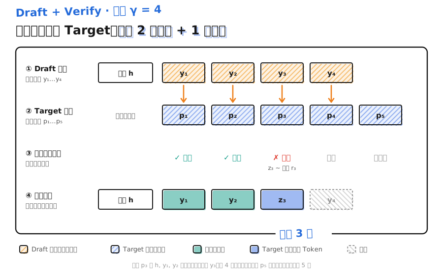
Example: Draft guessed 4 tokens; the first 2 pass and the 3rd is rejected. This round commits the first 2, then adds one token resampled by the rules at position 3; the 4th candidate is discarded. If all 4 pass, sample once more from , and the round advances 5 tokens in total.
The figure below draws the four steps of this round for that example (hatched yellow cells are uncommitted candidates, green are accepted, blue is the Target’s correction token, gray dashed cells are discarded):
3. Acceptance rules: greedy and random sampling differ
3.1 Greedy: compare against Target’s argmax
When the Target uses greedy decoding, the rule is simple: accept the -th candidate if it equals Target’s argmax at that position; otherwise replace it with Target’s argmax and end the round.
The resulting sequence matches Target’s own greedy decode exactly (assuming numerical agreement and consistent handling of tied maxima). It only applies when temperature is 0.
3.2 Random sampling: accept by probability ratio
When temperature is greater than 0, for a candidate drawn from , standard Speculative Sampling uses acceptance probability:
Intuitively: if Target likes this token at least as much as Draft (), always take it; if Target likes it less, accept with probability . In practice draw and accept when .
After rejection, do not simply redraw from . Sample from the residual distribution instead:
The residual keeps only the probability mass where Target wants the token more than Draft. Why this is required is in the section 4 proof; section 7 shows the consequence of doing it wrong in code.
3.3 When Draft gives only tokens, not probabilities
Methods like N-gram only emit tokens, with no probabilities; vLLM’s default for model Drafts, draft_sample_method="greedy", also takes only Draft’s argmax and does not keep the full Draft distribution. Then treat as a one-hot on the candidate: , and 0 elsewhere.
Plug into the formulas above and the acceptance probability becomes ; the residual after rejection is ” removed, renormalize the rest by .” The two paths still sum exactly to , so this remains lossless. The cost is that Draft’s probability information is unused, and acceptance rate depends on how much probability Target assigns to Draft’s preferred token. With "probabilistic", vLLM keeps Draft’s full probabilities for verification, at the cost of more GPU memory.
🔑 Core idea: the residual distribution compensates for probability mass the acceptance path over- or under-assigns. Acceptance rules and correction sampling must be used as a pair; changing only one of them changes the final distribution.
4. Correctness proof: both paths together equal Target
Fix one position and its history, and drop subscripts. The derivation matches Leviathan et al. and Chen et al.. A token is finally emitted on only two paths: Draft drew it and it was accepted, or after rejection it was drawn from the residual.
4.1 How much the accept path contributes
The joint probability of being drawn and then accepted is:
Write total acceptance probability , and rejection probability . Because and are normalized, , so:
That is exactly the residual distribution’s denominator.
4.2 The reject path fills the gap
After rejection, sampling from gives joint probability of outputting :
Add both paths:
Done. When , , the reject path is never taken, and a zero residual denominator never comes up.
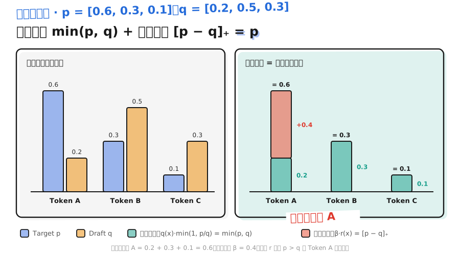
The figure below checks the identity with the same numbers as the section 7 experiment (left: blue bars , yellow bars ; right: green is the accept path , red is the reject path filling in ; stacked they equal ):
⚠️ Note: looking only at “accepted tokens,” they follow , which generally is not . What strictly follows Target is the combined final output of acceptance and correction.
4.3 Acceptance rate tracks how close the two distributions are
With total variation distance one can write:
The more Draft and Target overlap, the fewer corrections are needed. That is only the acceptance probability at one position under one history; how much faster a whole request gets is a separate cost ledger, which section 5.4 works through.
5. From one position to a full sequence
Every kept token is produced under the rules above on the true committed prefix, so by induction over positions the full sequence distribution matches Target:
5.1 Why you must stop after the first rejection
Suppose is rejected and replaced by . The already-computed was conditioned on , but the true history is now . The basis for checking is gone, even if “looks reasonable.”
So each round can only commit a contiguous accepted prefix; you cannot skip a wrong position and stitch later candidates. Draft Trees in section 5.3 keep only one legal path for the same reason.
5.2 Why you can get one bonus token
When all candidates pass, is already computed on the correct history, so sample from it directly; when something is rejected mid-round, add one correction token. Either way every round advances at least 1 and at most tokens.
EOS, stop strings, output length limits, or context limits can make the actual commit shorter. The engine truncates at the stop condition and does not cross it just to fill out a round.
6. KV Cache: drafts are not committed history
When candidates enter the Target forward pass, they occupy KV slots first. Until verification finishes, that KV is only a trial: rejected parts must be invalidated, or the next round will read history that never really happened.
| 📦 State | What to do | Common mistake |
|---|---|---|
| Committed history | Keep the matching KV | Rollback wrongly deletes prompt KV |
| Contiguously accepted candidates | Reuse the KV computed during verify | Run another forward and waste the gain |
| Rejected position and its suffix | Mark invalid, roll back the cache pointer | Next round still reads wrong-candidate KV |
| Correction / bonus token | Commit it, but compute its KV only when it is input next round | Treat “already sampled” as “already has KV” |
The last row is the easiest place for an off-by-one: the correction token is already emitted outward, but its own KV is only created when it becomes input to the next forward. So the engine must track committed token count and tokens with computed KV separately.
If Draft has its own KV Cache, it must also roll back to the finally committed history. Once Target vetoes , Draft’s next round must continue from , not along its original .
📌 Key point: the probability proof covers “how each token is sampled”; cache and scheduling cover “whether the next round sees the right history.” Misalignment on either side means theoretical losslessness never lands.
7. Hands-on: how wrong resampling changes the distribution
The code below uses only the Python standard library to simulate one position under a fixed history — no model load, no GPU timing. It compares three approaches: the standard rule, the wrong rule of redrawing from after reject, and the one-hot Draft from section 3.3.
import random
from collections import Counter

p = [0.6, 0.3, 0.1]  # Target
q = [0.2, 0.5, 0.3]  # Draft


def final_dist(p, q, resample):
    """Accept path min(p, q) + reject probability × post-reject sampling distribution."""
    overlap = [min(a, b) for a, b in zip(p, q)]
    beta = 1 - sum(overlap)
    return [o + beta * r for o, r in zip(overlap, resample)]


beta = sum(max(a - b, 0) for a, b in zip(p, q))
residual = [max(a - b, 0) / beta for a, b in zip(p, q)]
print("Standard rule:", final_dist(p, q, residual))
print("Wrong rule (redraw from p after reject):", final_dist(p, q, p))

# one-hot Draft: always proposes q's argmax (index 1, the second token); q collapses to [0, 1, 0]
q_onehot = [0.0, 1.0, 0.0]
beta1 = sum(max(a - b, 0) for a, b in zip(p, q_onehot))
residual1 = [max(a - b, 0) / beta1 for a, b in zip(p, q_onehot)]
exact = final_dist(p, q_onehot, residual1)
assert all(abs(a - b) < 1e-12 for a, b in zip(exact, p))
print("one-hot Draft:", exact, "acceptance rate:", 1 - beta1)

# Monte Carlo check of the standard rule
rng = random.Random(42)
counts, accepted, trials = Counter(), 0, 100_000
for _ in range(trials):
    y = rng.choices(range(3), weights=q)[0]
    if rng.random() < min(1, p[y] / q[y]):
        token, accepted = y, accepted + 1
    else:
        token = rng.choices(range(3), weights=residual)[0]
    counts[token] += 1
print("Empirical distribution:", [counts[i] / trials for i in range(3)], "acceptance rate:", accepted / trials)
Under the standard rule, the accept path contributes , and rejection probability 0.4 all goes to the first token, recovering . The wrong rule yields : the second and third tokens are overestimated by 40%, the first underestimated by about 27%. The one-hot Draft’s acceptance rate is only 0.3, but the final distribution is still — losslessness and acceptance rate are separate questions.
Monte Carlo will wobble by a few thousandths; it helps you see the proof, while correctness still rests on the exact calculation.
8. Engineering bounds: what lossless actually guarantees
“Lossless” is a precise mathematical promise; its scope has to be stated carefully:
- Guarantees matching distribution: correctly implemented speculative sampling matches the distribution of the Target being verified.
- Does not guarantee identical text: under random sampling, two execution paths consume randomness differently, so the same seed can still produce different text.
- Does not repair the Target itself: if Target is already quantized, the guarantee is relative to the quantized model, not an automatic restore to original BF16.
- Only covers the standard rules: threshold accept, Typical Acceptance, vLLM’s
syntheticmode for stress tests, and similar are out of scope and need separate quality evaluation.
History-dependent logits processors such as repetition penalty and structured output must also update state per candidate prefix during verification. Whether a framework supports a given combination depends on that version’s docs and tests.
vLLM docs split lossless into three layers: theoretically lossless (subject to hardware numeric precision), algorithmically covered by Rejection Sampler convergence tests and greedy consistency tests, and no promise of fully stable logprobs. Different batch shapes and kernels can swap two nearly tied logits, so you still need end-to-end output comparison before shipping.
📝 Summary
- Speculative decoding lets a cheap Draft write candidates, then one Target forward verifies them in batch; what shrinks is the number of serial Target rounds.
- What runs in parallel is conditional distributions over known candidates; the autoregressive dependence remains.
- Under greedy, compare argmax; under random sampling, accept with , and after reject sample from the normalized residual .
- The accept path contributes , the reject path fills , and together they equal .
- Token-only Drafts can be treated as one-hot and stay lossless; acceptance rate then depends on .
- Each round commits only a contiguous accepted prefix plus one new token; candidates after the first rejection are all discarded.
- KV rollback, Draft state sync, and logits processor state are the engineering half of whether losslessness lands.
- Lossless is relative to the actual Target; it is not identical text, and it is not a speed guarantee.
🎯 Self-check list
- Explain why known candidates can be verified in parallel, while unknown future tokens cannot be generated in parallel directly
- Mark which history and are each conditioned on
- Write both greedy and random-sampling acceptance rules
- Derive from the accept and reject paths that the final distribution equals
- Use a numeric example to show why redrawing from after reject is biased
- Explain why a one-hot Draft is still lossless
- Explain why the suffix after the first rejection must be dropped, and where the bonus token comes from
- Distinguish committed tokens, tokens with computed KV, and temporary candidates
- State the bounds of “lossless” under a quantized Target, the same seed, and approximate acceptance
📚 References
- Fast Inference from Transformers via Speculative Decoding (Leviathan et al., 2023)
- Accelerating Large Language Model Decoding with Speculative Sampling (Chen et al., 2023)
- vLLM — Speculative Decoding and lossless guarantees
- vLLM v0.32.0 — Rejection Sampler implementation
- vLLM v0.32.0 — SpeculativeConfig (draft_sample_method and related fields)