3.2 Transformer overview and code implementation
From the original Encoder-Decoder to Decoder-only evolution, with a full Transformer built from scratch in PyTorch
Before tearing Transformer into parts, step back and see the whole machine. This article starts from the 2017 Encoder-Decoder paper, walks through Encoder and Decoder internals and data flow, then follows three evolution paths (Encoder-only, Encoder-Decoder, Decoder-only), zooms in on today’s mainstream Decoder-only LLMs, and finally implements a full Encoder-Decoder Transformer in PyTorch so theory and code line up.
📑 Contents
- 1. Why look at the whole picture first
- 2. Original Transformer: Encoder-Decoder
- 3. Encoder internals
- 4. Decoder internals
- 5. Architecture evolution: three forks
- 6. Decoder-only: end-to-end structure of today’s LLMs
- 7. Reading real model structure from config
- 8. Engineering comparison of the three architectures
- 9. PyTorch implementation: build Transformer from scratch
- Summary
- Self-check list
- References
1. Why look at the whole picture first
The most common mistake when learning Transformer is diving straight into Self-Attention matmul details and ending up with trees but no forest — you know how is computed, but cannot say what steps the model takes from a sentence to the next word.
Analogy: the first time you walk into an unfamiliar factory, the useful move is not to crack open one gearbox on the line. Walk the floor first — where raw material enters, how many stations it passes, where finished goods leave. With that factory map, every machine you later open has a place and a job on the line.
This article is that map. After reading it you should know:
- What Encoder and Decoder each do in the original Transformer, and how they work together
- What each of the three variants (Encoder-only, Encoder-Decoder, Decoder-only) kept and cut
- The full data path of a modern LLM from token in to probability out
- Each component’s role end to end, so later deep dives have a coordinate system
2. Original Transformer: Encoder-Decoder
In 2017 Vaswani et al. published “Attention Is All You Need”: a sequence transduction model built entirely on attention, dropping the then-dominant RNN/LSTM. That is where Transformer begins.
2.1 Design motive: born for machine translation
The original Transformer targets sequence-to-sequence (Seq2Seq) — given an input sequence (e.g. an English sentence), produce an output sequence (e.g. a French translation). That naturally needs two stages: first understand the input, then generate the output. So the model splits into two symmetric halves:
- Encoder: compress the input sequence into a set of “understood” representations
- Decoder: from those representations, generate the output sequence step by step
Like how a human translates: read the English sentence once, form an understanding in your head (encode), then write the French word by word (decode), looking back at that understanding for every word.
2.2 Overall architecture
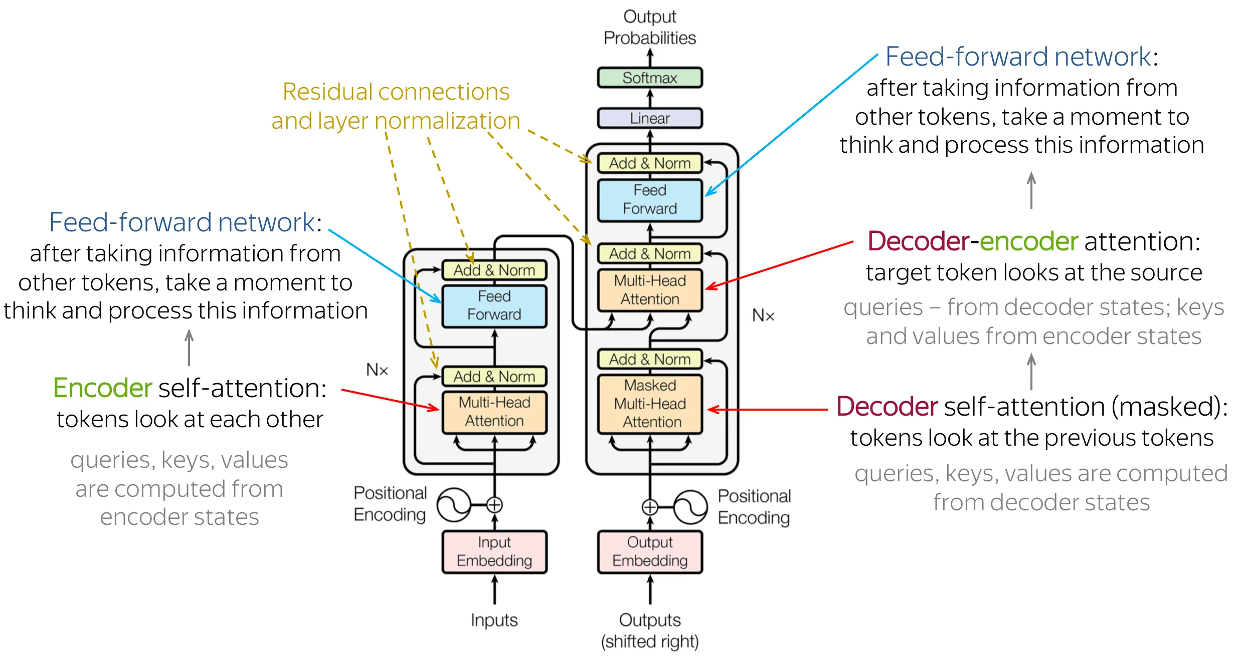
In the original paper, Encoder and Decoder each have layers, hidden size , attention heads, FFN inner size .
2.3 Division of labor among three attentions
The original Transformer uses three attentions. The underlying math is the same (Scaled Dot-Product Attention), but Q, K, V come from different places and play different roles:
| Attention type | Where | Q from | K, V from | Role |
|---|---|---|---|---|
| Encoder Self-Attention | Encoder layer | Input sequence | Input sequence | Tokens in the input exchange information |
| Masked Decoder Self-Attention | Decoder layer | Generated sequence so far | Generated sequence so far | Generated tokens exchange information (no looking ahead) |
| Cross-Attention | Decoder layer | Generated sequence so far | Encoder output | During generation, “look back” at the input |
In the translation metaphor:
- Encoder Self-Attention is reading the source and weighing how each word relates to the others
- Masked Decoder Self-Attention is reviewing what you have already written
- Cross-Attention is checking the source while writing the translation
3. Encoder internals
The Encoder’s job is to “read” the input. It takes a token sequence and emits a same-length contextual representation — each position’s output vector mixes information from the whole input.
3.1 Input processing
Before Encoder layers, the raw input goes through two steps:
Token Embedding: map each token ID to a dense -dim vector via a learnable embedding matrix , where is vocab size.
Positional Encoding: Attention itself has no position (shuffle tokens and the result is unchanged), so you inject position explicitly. The original paper uses sine/cosine encodings added onto token embeddings:
The processed input has shape , where is source length.
3.2 Data flow inside one Encoder layer
Each Encoder layer has two submodules; each is wrapped with residual connection and LayerNorm:
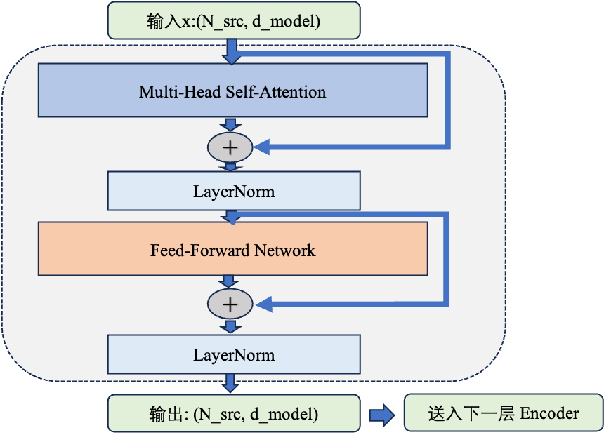
Note the original paper uses Post-Norm (sublayer first, then LayerNorm): . Modern LLMs mostly switched to Pre-Norm (LayerNorm first, then sublayer). Knowing the original design helps you track the evolution.
3.3 Key property of Encoder Self-Attention
Encoder Self-Attention is bidirectional — every token may attend to every other token, past and future.
As an attention mask (1 = allowed, shape ):
     t0  t1  t2  t3  t4
t0 [  1   1   1   1   1 ]
t1 [  1   1   1   1   1 ]
t2 [  1   1   1   1   1 ]
t3 [  1   1   1   1   1 ]
t4 [  1   1   1   1   1 ]
Fully connected — no masking. Even in the first Encoder layer, the last token can directly affect the first token’s representation. After N Encoder layers, each position’s output aggregates global information from the whole input.
3.4 Information flow across stacked layers
The original paper stacks 6 Encoder layers. The key design: every layer has identical input and output shape (both ). Layers stack like Lego — 6, 12, or 100, as long as memory fits.
Intuition for stacking: each layer does one round of “mix and refine.” Shallow layers may pick up lexical and syntactic relations (collocations, modifiers); deeper layers more abstract semantics (coreference, implied relations). More layers mean stronger capacity for complex relations, and compute grows linearly.
4. Decoder internals
The Decoder’s job is to “generate” the output. It has one more attention than the Encoder — Cross-Attention — to “look up” Encoder outputs.
4.1 Data flow inside one Decoder layer
Each Decoder layer has three submodules (one more Cross-Attention than Encoder):
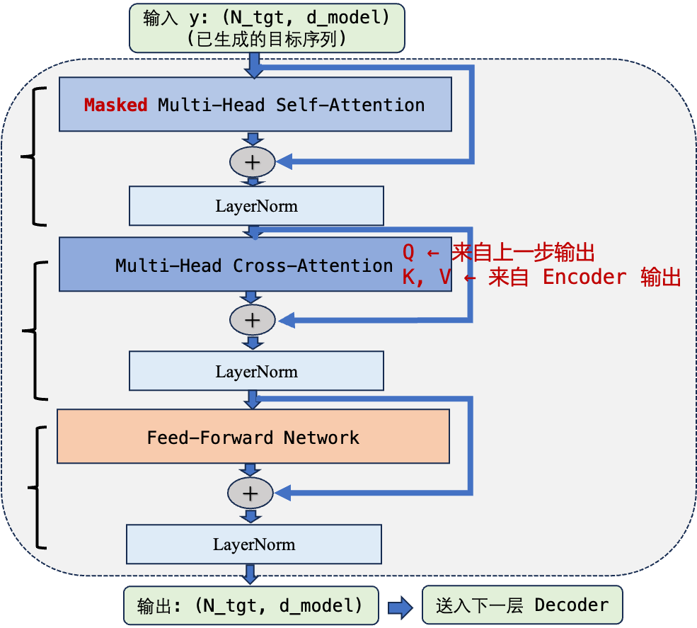
4.2 Masked Self-Attention: no peeking at the future
Decoder Self-Attention uses a Causal Mask so that when generating token you only see positions through , never beyond.
     t0  t1  t2  t3  t4
t0 [  1   0   0   0   0 ]    can only see itself
t1 [  1   1   0   0   0 ]    can see t0 and itself
t2 [  1   1   1   0   0 ]    can see t0, t1 and itself
t3 [  1   1   1   1   0 ]    can see everything before
t4 [  1   1   1   1   1 ]    can see all
That is a lower-triangular matrix. In practice you add an upper-triangular mask on the score matrix; after softmax those positions go to zero.
Why the mask? At train time, for speed, the whole target sequence is fed to the Decoder in parallel (Teacher Forcing). Without a mask, predicting word 3 could see words 4 and 5 — open-book exam; the model never learns to predict.
4.3 Cross-Attention: the bridge between Encoder and Decoder
Cross-Attention is the critical link in Encoder-Decoder. Compute is identical to Self-Attention; the only difference is where Q, K, V come from:
- Q (Query) from the current Decoder layer output — “what information do I want”
- K (Key) and V (Value) from the last Encoder layer — “what information does the source offer”
Shapes: if source length is and target length is :
- Attention score matrix: — not square!
No causal mask here: every Decoder token should attend to every Encoder position — when translating you need the full source.
4.4 Why three submodules in a Decoder layer
String the three together and each role is clear:
| Submodule | Input | Role | Analogy |
|---|---|---|---|
| Masked Self-Attention | Target sequence itself | Generated words coordinate — grammar and consistency | Reviewing paragraphs you already wrote |
| Cross-Attention | Target + source | Consult source while generating — stay faithful | Checking the original while writing the translation |
| FFN | Current token | Deep nonlinear processing of the combined signal | Digesting and forming your own wording |
Order matters: Self-Attention first integrates “context you already have,” Cross-Attention then adds “information from the input,” FFN finally does “deep processing.” That order means each token’s prediction sees both prior target context and the source.
5. Architecture evolution: three forks
After the original Transformer, researchers quickly saw Encoder and Decoder need not stay glued together. Depending on the task, you can keep only part of them. Three technical lines followed.
5.1 Encoder-only: the BERT line
In 2018 Google released BERT (Bidirectional Encoder Representations from Transformers): keep only the Encoder, drop Decoder and Cross-Attention.
Core idea: no generation; focus on “understanding.” BERT pretains with a Masked Language Model (hide some tokens, predict them) to get bidirectional language understanding.
Input: "The [MASK] sits on the mat"
      │
      ▼
  Encoder x 12 layers (bidirectional attention)
      │
      ▼
  Each position outputs a contextual representation
      │
      ▼
  [MASK] position → predict "cat" (pretrain)
  [CLS] position → class label (fine-tune)
Kept: bidirectional Self-Attention + FFN + residual + LayerNorm Cut: causal mask, Cross-Attention, autoregressive generation
Fit for: text classification, NER, sentence similarity, information extraction — anything that needs “understand” but not “generate.”
5.2 Encoder-Decoder: the T5 line
In 2019 Google released T5 (Text-to-Text Transfer Transformer), keeping full Encoder-Decoder but unifying the paradigm: cast every NLP task as text-to-text.
Classification: "classify: The movie is great" → "positive"
Translation:    "translate English to German: Hello" → "Hallo"
Summarization:  "summarize: [long text]" → "[summary]"
T5 showed that with a unified I/O format, one Encoder-Decoder can handle almost all NLP tasks. BART, mBART, UL2 and others followed this line.
Kept: full Encoder + Decoder + Cross-Attention Improved: unified text-to-text training format
5.3 Decoder-only: the GPT line
In 2018 OpenAI released GPT (Generative Pre-trained Transformer): keep only the Decoder (drop Cross-Attention), train with pure next-token prediction.
Input: "The cat sits on"
       │
       ▼
  Decoder x N layers (causal attention)
       │
       ▼
  Last position output → predict "the"
Kept: causal Self-Attention + FFN + residual + LayerNorm Cut: Encoder, Cross-Attention, bidirectional attention
From GPT-1 to GPT-4, from LLaMA to Mistral, Qwen, DeepSeek, Decoder-only became the absolute mainstream of the LLM era. The next section digs into its full structure.
6. Decoder-only: end-to-end structure of today’s LLMs
Decoder-only drops Encoder and Cross-Attention. The whole model fits a short formula: input tokens → Embedding → N Decoder Blocks → predict next token.
6.1 End-to-end data flow
Follow one real LLM inference from input to output:
User input: "什么是注意力机制"

Step 1: Tokenizer
────────────────────
"什么是注意力机制" → [1234, 567, 89, 2345, 678]  (5 token IDs)

Step 2: Token Embedding
────────────────────
[1234, 567, 89, 2345, 678]
    │
    ▼
W_embed: (vocab_size, d_model)   lookup vector per token
    │
    ▼
X: (5, d_model)                  5 d_model-dim vectors

Step 3: L Decoder Blocks
────────────────────
┌─ Block 1 ─────────────────────────────────────────────┐
│                                                       │
│  x_norm = RMSNorm(X)                                  │
│  attn_out = MaskedSelfAttention(x_norm)  ← with RoPE  │
│  H = X + attn_out                        ← residual   │
│                                                       │
│  h_norm = RMSNorm(H)                                  │
│  ffn_out = SwiGLU_FFN(h_norm)                         │
│  X = H + ffn_out                         ← residual   │
│                                                       │
└───────────────────────────────────────────────────────┘
    │                          shape stays (5, d_model)
    ▼
┌─ Block 2 ─────────── ... ───────── Block L ────────────┐
│                                                        │
│  Identical structure, repeated L times                 │
│                                                        │
└────────────────────────────────────────────────────────┘
    │
    ▼
X_final: (5, d_model)

Step 4: Final LayerNorm
────────────────────
X_norm = RMSNorm(X_final)        (5, d_model)

Step 5: LM Head
────────────────────
logits = X_norm @ W_lm_head      (5, d_model) × (d_model, vocab_size)
                                 = (5, vocab_size)

Step 6: Take last position, Softmax → sample
────────────────────
logits[-1]: (vocab_size,)         output at the last token position
    │
    ▼
probabilities = Softmax(logits[-1])
    │
    ▼
next_token = Sample(probabilities)  → e.g. sample "注"

Step 7: Autoregressive loop
────────────────────
Append the new token to the input, repeat Steps 2–6
"什么是注意力机制" + "注" → "什么是注意力机制注"
Keep generating... "意" → "力" → "机" → "制" → "是" → ...
Compact math form:
6.2 Five components
Split a Decoder-only model into five functional pieces end to end:
(1) Token Embedding
Like a word–vector dictionary. The model keeps ; a token ID indexes one row.
- LLaMA-2-7B: , , so has parameters
- Against 6.7B total, Embedding is only ~2%
(2) Stacked Decoder Blocks
The “body” of the model: 95%+ of parameters and compute. Block internals are covered in the intro piece and later deep dives; here the global properties matter:
- Shape conservation: every Block I/O is strictly , so Blocks stack freely
- No parameter sharing: each layer’s are independent; layers do not share weights
- Depth from layer count: LLaMA-2-7B has 32 layers, LLaMA-2-70B has 80; more layers means a “deeper” model that can in theory capture more complex patterns
(3) Final LayerNorm
After the last Decoder Block there is one more normalization. It stabilizes the numeric range before the LM Head so deep-network drift does not scramble the output distribution.
(4) LM Head
A simple linear layer maps -dim hidden states to vocab-sized logits.
One important engineering trick: Weight Tying. Some models (e.g. GPT-2) reuse the Token Embedding matrix for the LM Head (transposed): . At LLaMA-2-7B scale that would save 131M parameters (LLaMA-2 itself does not share; the two are independent), and it is semantically natural — mapping vectors back to tokens and tokens to vectors should be inverse operations.
(5) Softmax + sampling
Turn logits into a distribution, then pick the next token with a strategy (Greedy, Top-k, Top-p, Temperature, …). Strategy strongly affects quality and diversity — higher Temperature is more random; lower is more deterministic.
6.3 Structural contrast with original Encoder-Decoder
Side by side, what Decoder-only simplifies:
| Component | Encoder-Decoder | Decoder-only |
|---|---|---|
| Token Embedding | One each for Encoder and Decoder | Only one |
| Positional Encoding | Additive (Sinusoidal) | Rotary (RoPE, applied at Attention time) |
| Self-Attention | Encoder: bidirectional / Decoder: causal | Causal Self-Attention only |
| Cross-Attention | Yes (every Decoder layer) | None |
| FFN | In both Encoder and Decoder | One per layer |
| LayerNorm placement | Post-Norm | Pre-Norm (most LLMs) |
| Normalization | LayerNorm | RMSNorm (most LLMs) |
| Output head | Linear + Softmax | Linear + Softmax (may Weight Tie) |
7. Reading real model structure from config
With the architecture clear, look at real open-model configs and map abstract structure to numbers.
7.1 LLaMA-2 family
| Config | 7B | 13B | 70B |
|---|---|---|---|
| (hidden size) | 4096 | 5120 | 8192 |
| (layers) | 32 | 40 | 80 |
| (attention heads) | 32 | 40 | 64 |
| (per-head dim) | 128 | 128 | 128 |
| (FFN inner dim) | 11008 | 13824 | 28672 |
| vocab_size | 32000 | 32000 | 32000 |
| Total params | 6.7B | 13B | 70B |
| Positional encoding | RoPE | RoPE | RoPE |
| Normalization | RMSNorm | RMSNorm | RMSNorm |
| FFN activation | SwiGLU | SwiGLU | SwiGLU |
| KV heads | 32 (MHA) | 40 (MHA) | 8 (GQA) |
One key difference at 70B: it uses GQA (Grouped-Query Attention) with only 8 KV heads (not 64), so every 8 Q heads share one KV group and inference KV Cache cost drops sharply.
7.2 Reconstructing structure from config
Given a config you can rebuild the compute graph. For LLaMA-2-7B, layer by layer:
Input: token_ids (batch, seq_len)
  │
  ▼
Token Embedding: (32000, 4096)          ← 131M params
  │
  ▼
═══════════ Decoder Block × 32 layers ═══════════
  Each layer contains:
  ├─ RMSNorm_1: (4096,)                ← 4K params
  ├─ W_Q: (4096, 4096)                 ← 16.8M params
  ├─ W_K: (4096, 4096)                 ← 16.8M params
  ├─ W_V: (4096, 4096)                 ← 16.8M params
  ├─ W_O: (4096, 4096)                 ← 16.8M params
  ├─ RMSNorm_2: (4096,)                ← 4K params
  ├─ W_gate: (4096, 11008)             ← 45.1M params
  ├─ W_up:   (4096, 11008)             ← 45.1M params
  └─ W_down: (11008, 4096)             ← 45.1M params

  Per layer total: ~201M params
  32 layers total: ~6,432M params
═══════════════════════════════════════════════
  │
  ▼
Final RMSNorm: (4096,)                  ← 4K params
  │
  ▼
LM Head: (4096, 32000)                  ← 131M params (independent, not shared with Embedding)
  │
  ▼
Output: logits (batch, seq_len, 32000)
Parameter split: 32 Decoder Blocks hold 6,432M / 6,738M 95.5% of parameters. Almost all of the model’s “knowledge” lives in those Block weight matrices.
7.3 Scale vs depth/width
You can grow a model two ways — deeper (more layers ) or wider (larger ). Rough parameter formula:
Here is one Decoder Block (4 Attention matrices + SwiGLU’s 3 matrices ≈ ), and is Embedding + LM Head (LLaMA does not share; if you tie embeddings like GPT-2 or Gemma, count only one ).
From the table:
- 7B → 13B: layers 32 → 40 (+25%), width 4096 → 5120 (+25%), params roughly double
- 13B → 70B: layers 40 → 80 (+100%), width 5120 → 8192 (+60%), params grow 5.4×
Params scale quadratically with width and linearly with depth, so widening grows parameters faster than deepening.
AI Infra note: that quadratic directly hits memory planning and parallel strategy. Double the width and per-layer params grow 4×; one GPU may not hold a single layer — then you need Tensor Parallelism to split inside a layer. Double the layers and Pipeline Parallelism can split across layers. Real deployments usually need both.
8. Engineering comparison of the three architectures
From an AI Infra view, the three architectures differ a lot in system design.
8.1 Compute characteristics
| Dimension | Encoder-only | Encoder-Decoder | Decoder-only |
|---|---|---|---|
| Attention complexity | , N = input length | Encoder: + Cross: + Decoder: | , N = total sequence length |
| Inference mode | Single forward (non-autoregressive) | Autoregressive (Decoder part) | Autoregressive |
| KV Cache | Not needed (no generation) | Encoder KV + Decoder KV | One Decoder KV |
| Typical latency | Milliseconds (classification) | Higher (two components) | Depends on generation length |
8.2 Parallelism differences
| Parallelism | Encoder-Decoder | Decoder-only |
|---|---|---|
| Tensor parallelism (TP) | Encoder and Decoder each need splits; Cross-Attention KV comes from Encoder, communication is more complex | Uniform layer structure, one split scheme, simple communication |
| Pipeline parallelism (PP) | Decide how many stages each of Encoder/Decoder gets; load balance is harder | All layers identical; even splits work |
| Sequence parallelism (SP) | Two sides may have different lengths; handle separately | One sequence dimension; uniform handling |
8.3 Why Decoder-only is friendliest for engineering
Beyond model quality, Decoder-only won the LLM era for deep engineering reasons:
Architectural uniformity. The whole model is one Block type stacked repeatedly, which means:
- CUDA kernels need only one set optimized (same Attention kernel, same FFN kernel reused L times)
- Parallel strategy designed once (no separate Encoder/Decoder scheduling)
- Profiling and bottleneck hunting are simpler (any layer represents all layers)
Simple KV Cache management. One KV Cache to manage; PagedAttention-style optimizations apply directly, with no second cache for Encoder outputs plus Decoder KV.
Clear scaling path. Want a bigger model? Add layers, width, heads — three knobs with predictable effect. No Encoder/Decoder ratio puzzle.
High training-data utilization. Next-token prediction gives a training signal (loss) at every token; utilization is near 100%. Encoder-Decoder only produces loss on the Decoder side; Encoder gradients come only by backprop from Decoder loss.
9. PyTorch implementation: build Transformer from scratch
After the theory, the best check is to write it yourself. This chapter implements a full Encoder-Decoder Transformer in PyTorch from scratch; every module maps to the structure diagrams above.
Dependencies:
import numpy as np
import torch
import torch.nn as nn
9.1 Masking: three Mask implementations
Masks are where implementations go wrong most often. There are three, matching the three attentions in section 2.
Encoder length Mask: samples in a batch are padded to the same length; Attention weights on padding must be blocked. Fill those scores with -1e4 so softmax drives them near 0.
def get_len_mask(b: int, max_len: int, feat_lens: torch.Tensor, device: torch.device) -> torch.Tensor:
    """Build the length mask for Encoder self-attention.
    Returns: shape (b, max_len, max_len); True means the position should be masked
    """
    attn_mask = torch.ones((b, max_len, max_len), device=device)
    for i in range(b):
        attn_mask[i, :, :feat_lens[i]] = 0
    return attn_mask.to(torch.bool)
Decoder Causal Mask: at train time the whole target is fed in parallel, but predicting position may only see through , enforced with an upper-triangular mask.
def get_subsequent_mask(b: int, max_len: int, device: torch.device) -> torch.Tensor:
    """Build the causal mask for Decoder self-attention (upper-triangular).
    Returns: shape (b, max_len, max_len); True means future positions (to mask)
    """
    return torch.triu(torch.ones((b, max_len, max_len), device=device), diagonal=1).to(torch.bool)
torch.triu(..., diagonal=1) keeps the strict upper triangle (); row may only attend to columns through .
Encoder-Decoder Cross-Attention Mask: in each Decoder Cross-Attention, K/V come from the Encoder; padding in Encoder outputs must be masked.
def get_enc_dec_mask(
    b: int,
    max_feat_len: int,
    feat_lens: torch.Tensor,
    max_label_len: int,
    device: torch.device,
) -> torch.Tensor:
    """Build the Encoder-Decoder Cross-Attention mask.
    Returns: shape (b, max_label_len, max_feat_len); True means Encoder padding positions
    """
    attn_mask = torch.zeros((b, max_label_len, max_feat_len), device=device)
    for i in range(b):
        attn_mask[i, :, feat_lens[i]:] = 1
    return attn_mask.to(torch.bool)
Comparing the three Masks:
| Mask type | Used where | Shape | Purpose |
|---|---|---|---|
| Length Mask | Encoder self-attention | (b, enc_len, enc_len) | Mask Encoder padding |
| Causal Mask | Decoder self-attention | (b, dec_len, dec_len) | Block future tokens |
| Cross-Attn Mask | Decoder Cross-Attention | (b, dec_len, enc_len) | Mask Encoder padding |
⚠️ Note: this article uses masked_fill_(mask, -1e4), where True means masked. PyTorch 2.0 scaled_dot_product_attention with a bool mask has the same semantics (True = masked); with a float mask the values are added to scores (large negatives act as masks).
9.2 Multi-Head Attention
Matches the Scaled Dot-Product Attention formula in section 3:
Four steps: linear projection → split heads → Scaled Dot-Product Attention → merge output.
class MultiHeadAttention(nn.Module):
    def __init__(self, d_k, d_v, d_model, num_heads, p=0.):
        """
        Args:
            d_k: Key/Query dim per attention head
            d_v: Value dim per attention head
            d_model: total input/output dim
            num_heads: number of attention heads
        """
        super(MultiHeadAttention, self).__init__()
        self.d_k = d_k
        self.d_v = d_v
        self.d_model = d_model
        self.num_heads = num_heads
        self.dropout = nn.Dropout(p)

        # Four linear projections: Q, K, V, and output
        self.W_Q = nn.Linear(d_model, d_k * num_heads)
        self.W_K = nn.Linear(d_model, d_k * num_heads)
        self.W_V = nn.Linear(d_model, d_v * num_heads)
        self.W_out = nn.Linear(d_v * num_heads, d_model)

        # Weight init (He-initialization style)
        nn.init.normal_(self.W_Q.weight, mean=0, std=np.sqrt(2.0 / (d_model + d_k)))
        nn.init.normal_(self.W_K.weight, mean=0, std=np.sqrt(2.0 / (d_model + d_k)))
        nn.init.normal_(self.W_V.weight, mean=0, std=np.sqrt(2.0 / (d_model + d_v)))
        nn.init.normal_(self.W_out.weight, mean=0, std=np.sqrt(2.0 / (d_model + d_v)))

    def forward(self, Q, K, V, attn_mask):
        """
        Args:
            Q: (batch, q_len, d_model)
            K: (batch, k_len, d_model)
            V: (batch, v_len, d_model)  note k_len == v_len
            attn_mask: (batch, q_len, k_len) or None
        Returns:
            output: (batch, q_len, d_model)
        """
        N = Q.size(0)
        q_len, k_len = Q.size(1), K.size(1)
        d_k, d_v, num_heads = self.d_k, self.d_v, self.num_heads

        # Step 1: linear projection + split heads
        # (N, q_len, d_model) -> (N, num_heads, q_len, d_k)
        Q = self.W_Q(Q).view(N, -1, num_heads, d_k).transpose(1, 2)
        K = self.W_K(K).view(N, -1, num_heads, d_k).transpose(1, 2)
        V = self.W_V(V).view(N, -1, num_heads, d_v).transpose(1, 2)

        # Step 2: broadcast Mask to the head dim
        if attn_mask is not None:
            assert attn_mask.size() == (N, q_len, k_len)
            attn_mask = attn_mask.unsqueeze(1).repeat(1, num_heads, 1, 1).bool()

        # Step 3: Scaled Dot-Product Attention
        scores = torch.matmul(Q, K.transpose(-1, -2)) / np.sqrt(d_k)
        if attn_mask is not None:
            scores.masked_fill_(attn_mask, -1e4)
        attns = torch.softmax(scores, dim=-1)
        attns = self.dropout(attns)

        # Step 4: weighted sum + merge heads + output projection
        output = torch.matmul(attns, V)
        output = output.transpose(1, 2).contiguous().reshape(N, -1, d_v * num_heads)
        output = self.W_out(output)
        return output
💡 Tip: the paper’s standard config is , , , so and I/O dims match.
9.3 Sinusoidal positional encoding
Matches the Positional Encoding design in §3.1; implements the paper’s sine/cosine formulas:
def pos_sinusoid_embedding(seq_len: int, d_model: int) -> torch.Tensor:
    """Build a sine/cosine positional encoding matrix (not learnable; frozen).
    Returns: (seq_len, d_model)
    """
    embeddings = torch.zeros((seq_len, d_model))
    for i in range(d_model):
        f = torch.sin if i % 2 == 0 else torch.cos
        embeddings[:, i] = f(
            torch.arange(0, seq_len) / np.power(1e4, 2 * (i // 2) / d_model)
        )
    return embeddings.float()
In Encoder/Decoder, nn.Embedding.from_pretrained(..., freeze=True) freezes positional encodings as non-trainable parameters and indexes them by position at use time.
9.4 Position-wise FFN
Matches the FFN submodule of the Encoder layer in §3.2: a two-layer MLP applied independently per token:
Implemented with nn.Linear on the last dim; no transpose needed:
class PoswiseFFN(nn.Module):
    def __init__(self, d_model: int, d_ff: int, p: float = 0.):
        """d_ff is usually 4 * d_model (e.g. d_model=512 → d_ff=2048)"""
        super(PoswiseFFN, self).__init__()
        self.fc1 = nn.Linear(d_model, d_ff)
        self.fc2 = nn.Linear(d_ff, d_model)
        self.relu = nn.ReLU(inplace=True)
        self.dropout = nn.Dropout(p=p)

    def forward(self, X):
        # X: (N, seq_len, d_model)
        out = self.fc1(X)          # -> (N, seq_len, d_ff)
        out = self.relu(out)
        out = self.fc2(out)        # -> (N, seq_len, d_model)
        return self.dropout(out)
9.5 EncoderLayer and Encoder
EncoderLayer matches the data-flow diagram in §3.2: Multi-Head Self-Attention + FFN, each sublayer wrapped with residual and LayerNorm (Post-Norm style).
class EncoderLayer(nn.Module):
    def __init__(self, dim: int, n: int, dff: int, dropout_posffn: float, dropout_attn: float):
        assert dim % n == 0
        super(EncoderLayer, self).__init__()
        hdim = dim // n  # dim per attention head

        self.norm1 = nn.LayerNorm(dim)
        self.norm2 = nn.LayerNorm(dim)
        self.multi_head_attn = MultiHeadAttention(hdim, hdim, dim, n, dropout_attn)
        self.poswise_ffn = PoswiseFFN(dim, dff, p=dropout_posffn)

    def forward(self, enc_in, attn_mask):
        # Self-Attention: Q=K=V=enc_in (bidirectional attention in §3.3)
        residual = enc_in
        context = self.multi_head_attn(enc_in, enc_in, enc_in, attn_mask)
        out = self.norm1(residual + context)   # residual + LayerNorm

        # FFN
        residual = out
        out = self.poswise_ffn(out)
        out = self.norm2(residual + out)       # residual + LayerNorm
        return out
Full Encoder: N EncoderLayers after adding positional encodings.
class Encoder(nn.Module):
    def __init__(self, dropout_emb, dropout_posffn, dropout_attn,
                 num_layers, enc_dim, num_heads, dff, tgt_len):
        super(Encoder, self).__init__()
        self.tgt_len = tgt_len
        # Fixed sinusoidal positional encoding (freeze=True: no grad updates)
        self.pos_emb = nn.Embedding.from_pretrained(
            pos_sinusoid_embedding(tgt_len, enc_dim), freeze=True
        )
        self.emb_dropout = nn.Dropout(dropout_emb)
        self.layers = nn.ModuleList(
            [EncoderLayer(enc_dim, num_heads, dff, dropout_posffn, dropout_attn)
             for _ in range(num_layers)]
        )

    def forward(self, X, X_lens, mask=None):
        # X: (batch, seq_len, d_model)
        seq_len = X.size(1)
        out = X + self.pos_emb(torch.arange(seq_len, device=X.device))  # add positional encoding
        out = self.emb_dropout(out)
        for layer in self.layers:
            out = layer(out, mask)
        return out
9.6 DecoderLayer and Decoder
DecoderLayer matches the data-flow diagram in §4.1: three sublayers — Masked Self-Attention → Cross-Attention → FFN.
class DecoderLayer(nn.Module):
    def __init__(self, dim: int, n: int, dff: int, dropout_posffn: float, dropout_attn: float):
        assert dim % n == 0
        super(DecoderLayer, self).__init__()
        hdim = dim // n

        self.norm1 = nn.LayerNorm(dim)
        self.norm2 = nn.LayerNorm(dim)
        self.norm3 = nn.LayerNorm(dim)
        self.poswise_ffn = PoswiseFFN(dim, dff, p=dropout_posffn)
        self.dec_attn = MultiHeadAttention(hdim, hdim, dim, n, dropout_attn)     # Masked Self-Attn
        self.enc_dec_attn = MultiHeadAttention(hdim, hdim, dim, n, dropout_attn) # Cross-Attn

    def forward(self, dec_in, enc_out, dec_mask, dec_enc_mask):
        """
        dec_in:       (batch, dec_len, d_model)  current Decoder layer input
        enc_out:      (batch, enc_len, d_model)  final Encoder output
        dec_mask:     Causal Mask (batch, dec_len, dec_len)
        dec_enc_mask: Cross-Attn Mask (batch, dec_len, enc_len)
        """
        # 1. Masked Self-Attention (see §4.2)
        residual = dec_in
        context = self.dec_attn(dec_in, dec_in, dec_in, dec_mask)
        dec_out = self.norm1(residual + context)

        # 2. Cross-Attention (see §4.3): Q from Decoder, K/V from Encoder
        residual = dec_out
        context = self.enc_dec_attn(dec_out, enc_out, enc_out, dec_enc_mask)
        dec_out = self.norm2(residual + context)

        # 3. FFN
        residual = dec_out
        out = self.poswise_ffn(dec_out)
        dec_out = self.norm3(residual + out)
        return dec_out
Full Decoder: Word Embedding on the target, add positional encoding, then decode layer by layer.
class Decoder(nn.Module):
    def __init__(self, dropout_emb, dropout_posffn, dropout_attn,
                 num_layers, dec_dim, num_heads, dff, tgt_len, tgt_vocab_size):
        super(Decoder, self).__init__()
        # Word Embedding: map token IDs to d_model-dim vectors
        self.tgt_emb = nn.Embedding(tgt_vocab_size, dec_dim)
        self.dropout_emb = nn.Dropout(p=dropout_emb)
        # Fixed sinusoidal positional encoding
        self.pos_emb = nn.Embedding.from_pretrained(
            pos_sinusoid_embedding(tgt_len, dec_dim), freeze=True
        )
        self.layers = nn.ModuleList(
            [DecoderLayer(dec_dim, num_heads, dff, dropout_posffn, dropout_attn)
             for _ in range(num_layers)]
        )

    def forward(self, labels, enc_out, dec_mask, dec_enc_mask):
        # labels: (batch, dec_len) token ID sequence
        tgt_emb = self.tgt_emb(labels)
        pos_emb = self.pos_emb(torch.arange(labels.size(1), device=labels.device))
        dec_out = self.dropout_emb(tgt_emb + pos_emb)
        for layer in self.layers:
            dec_out = layer(dec_out, enc_out, dec_mask, dec_enc_mask)
        return dec_out
9.7 Assemble the full Transformer
Combine Frontend (input feature transform), Encoder, Decoder, and LM Head into the full model, matching the overall architecture in §2.2:
class Transformer(nn.Module):
    def __init__(self, frontend: nn.Module, encoder: Encoder,
                 decoder: Decoder, dec_out_dim: int, vocab: int):
        """
        frontend:    input feature transform (e.g. linear fbank_dim → d_model)
        dec_out_dim: Decoder output dim (= d_model)
        vocab:       target vocab size
        """
        super().__init__()
        self.frontend = frontend
        self.encoder = encoder
        self.decoder = decoder
        self.linear = nn.Linear(dec_out_dim, vocab)  # LM Head

    def forward(self, X: torch.Tensor, X_lens: torch.Tensor, labels: torch.Tensor):
        """
        X:      (batch, enc_len, fbank_dim)  input feature sequence
        X_lens: (batch,)                      actual input length per sample
        labels: (batch, dec_len)              target token ID sequence
        Returns: logits (batch, dec_len, vocab_size)
        """
        X_lens, labels = X_lens.long(), labels.long()
        b, device = X.size(0), X.device

        # Frontend + Encoder (Encoder structure in §3)
        out = self.frontend(X)
        max_feat_len = out.size(1)
        enc_mask = get_len_mask(b, max_feat_len, X_lens, device)
        enc_out = self.encoder(out, X_lens, enc_mask)

        # Decoder (Decoder structure in §4)
        max_label_len = labels.size(1)
        dec_mask = get_subsequent_mask(b, max_label_len, device)
        dec_enc_mask = get_enc_dec_mask(b, max_feat_len, X_lens, max_label_len, device)
        dec_out = self.decoder(labels, enc_out, dec_mask, dec_enc_mask)

        # LM Head
        return self.linear(dec_out)
9.8 Forward check
Validate the full forward pass with random dummy data:
if __name__ == "__main__":
    batch_size    = 16
    max_feat_len  = 100    # max Encoder input length
    max_label_len = 50     # max Decoder target length
    fbank_dim     = 80     # input feature dim (e.g. 80-dim Fbank)
    hidden_dim    = 512    # d_model
    vocab_size    = 26     # vocab size

    fbank_feature = torch.randn(batch_size, max_feat_len, fbank_dim)
    feat_lens     = torch.randint(1, max_feat_len, (batch_size,))
    labels        = torch.randint(0, vocab_size, (batch_size, max_label_len))

    feature_extractor = nn.Linear(fbank_dim, hidden_dim)
    encoder = Encoder(
        dropout_emb=0.1, dropout_posffn=0.1, dropout_attn=0.,
        num_layers=6, enc_dim=hidden_dim, num_heads=8, dff=2048, tgt_len=2048,
    )
    decoder = Decoder(
        dropout_emb=0.1, dropout_posffn=0.1, dropout_attn=0.,
        num_layers=6, dec_dim=hidden_dim, num_heads=8, dff=2048,
        tgt_len=2048, tgt_vocab_size=vocab_size,
    )
    model = Transformer(feature_extractor, encoder, decoder, hidden_dim, vocab_size)

    logits = model(fbank_feature, feat_lens, labels)
    print(f"logits shape: {logits.shape}")
    # output: logits shape: torch.Size([16, 50, 26])
logits has shape (batch_size, dec_len, vocab_size): the vocab distribution at each decode step. Attach cross-entropy loss and you can train.
📝 Summary
A one-table recap of the core content:
| Topic | Takeaway |
|---|---|
| Original Transformer | Encoder-Decoder, designed for Seq2Seq (translation) |
| Three attentions | Encoder Self-Attention (bidirectional), Masked Decoder Self-Attention (causal), Cross-Attention (cross-sequence) |
| Encoder | Bidirectional attention + FFN; contextual representations of the input |
| Decoder | Causal Self-Attention + Cross-Attention + FFN; autoregressive generation |
| Three evolution lines | Encoder-only (BERT), Encoder-Decoder (T5), Decoder-only (GPT/LLaMA) |
| Decoder-only structure | Embedding → L Decoder Blocks → Final Norm → LM Head → Softmax |
| Decoder-only advantages | Unified training objective, simple engineering, clear Scaling, simple KV Cache |
| Code | Three Masks → MultiHeadAttention → sinusoidal PE → FFN → EncoderLayer → DecoderLayer → Transformer |
From the overview, Transformer’s design philosophy fits in three lines:
- Attention handles information exchange — tokens pass information to each other
- FFN handles information processing — nonlinear transforms per token independently
- Residual + normalization keep training stable — so deep stacks can train
Those three pillars plus “stacking” (repeat the same Block N times) are the whole essence of Transformer. When you deep-dive individual modules later, come back to this map and check where the part sits in the machine.
🎯 Self-check list
- Draw the original Encoder-Decoder overview; mark where the three attentions sit and where Q/K/V come from
- Explain roles and differences of Encoder Self-Attention, Masked Decoder Self-Attention, and Cross-Attention
- Say what Encoder-only, Encoder-Decoder, and Decoder-only each kept and cut from the original Transformer
- Describe end-to-end Decoder-only LLM inference: token ID → Embedding → N Blocks → Norm → LM Head → Softmax → sample
- Recite the five Decoder-only components (Embedding, Block stack, Final Norm, LM Head, Softmax) and each role
- Given config params (, , vocab_size, …), estimate total parameter count
- Explain what Weight Tying means and why it helps in engineering
- From an engineering angle, give at least three reasons Decoder-only is friendlier for AI Infra
- Name the three Masks, where they are used, and their shapes (
(b, q_len, k_len)) - Explain why Causal Mask is upper-triangular and what
torch.triu(..., diagonal=1)means - Describe Multi-Head Attention’s four steps: linear projection → split heads → Scaled Dot-Product Attention → merge output
- Write the sinusoidal PE formulas and explain why Transformer needs explicit position while RNN does not
- Run the full forward check and explain what the
logitsdims mean
📚 References
- Attention Is All You Need (Vaswani et al., 2017) — Original Transformer paper; full Encoder-Decoder and sinusoidal PE
- BERT: Pre-training of Deep Bidirectional Transformers (Devlin et al., 2018) — Founding Encoder-only work
- Exploring the Limits of Transfer Learning with a Unified Text-to-Text Transformer (Raffel et al., 2019) — T5; unified Encoder-Decoder paradigm
- Language Models are Unsupervised Multitask Learners (Radford et al., 2019) — GPT-2; foundation of Decoder-only
- LLaMA: Open and Efficient Foundation Language Models (Touvron et al., 2023) — LLaMA architecture and configs
- Sequence to Sequence Learning with Neural Networks (Sutskever et al., 2014) — Foundational Encoder-Decoder paper
- Are Sixteen Heads Really Better than One? (Michel et al., 2019) — Empirical analysis of multi-head attention
- The Illustrated Transformer (Jay Alammar) — Visual Transformer intro
- The Annotated Transformer (Harvard NLP) — Paper line-by-line with PyTorch
- PyTorch nn.MultiheadAttention — Official Multi-Head Attention docs