6.2 Tensor-parallel inference
From Megatron column/row splits, derive TP inference's two AllReduces per layer—volume and latency—then analyze GQA KV-head replication, NVLink dependence, how TP degree affects latency vs throughput differently, and vLLM's Custom AllReduce
Section 6.1 said that, unlike PP, TP lets several cards compute the same token at once, so it is the first choice for cutting single-request latency. The cost is syncing every layer. This section first clears the per-layer split and the two AllReduces, then does the communication ledger, and finally discusses how large TP should be and why TP almost never crosses nodes.
Chapter 3 section 3.3 already walked ColumnParallelLinear and RowParallelLinear in nano-vllm. Here we look from a deployer’s view at what those splits mean on real models and hardware.
⏰ Currency: The principles do not depend on any framework; vLLM descriptions follow v0.32.0 (released 2026-10-18). Hardware bandwidth figures are from NVIDIA product pages.
📑 Contents
- 1. How one layer splits: column and row pairs
- 2. Attention by heads: KV-head replication under GQA
- 3. Communication ledger: how long two AllReduces take
- 4. Why TP stays inside a node
- 5. TP degree: separate latency from throughput
- 6. TP implementation details in vLLM
- 7. Hands-on: a rough model of TP degree vs time per token
- Summary
- Self-check list
- References
1. How one layer splits: column and row pairs
A Transformer layer has two sublayers: attention and FFN. TP’s split comes from the Megatron-LM paper; the core idea is to pair column splits with row splits.
Take FFN. Input , FFN is , with , .
- First matrix, column-split: ; card computes . The activation is elementwise, so each card owns its columns and the result is correct with no communication.
- Second matrix, row-split: is cut along into ; card computes , a full-shape partial sum.
Summing the partial sums is one AllReduce. Activations on the intermediate dim stay on each card and are never fully assembled.
Attention is the same pattern: QKV projections column-split by head; each card runs full attention on its heads; output projection o_proj is row-split, then another AllReduce. So each layer has exactly 2 AllReduces.
The figure below is one Llama-3.1-70B layer at TP=4; four colors are the four GPUs’ shards; purple bars are AllReduces that need every card:
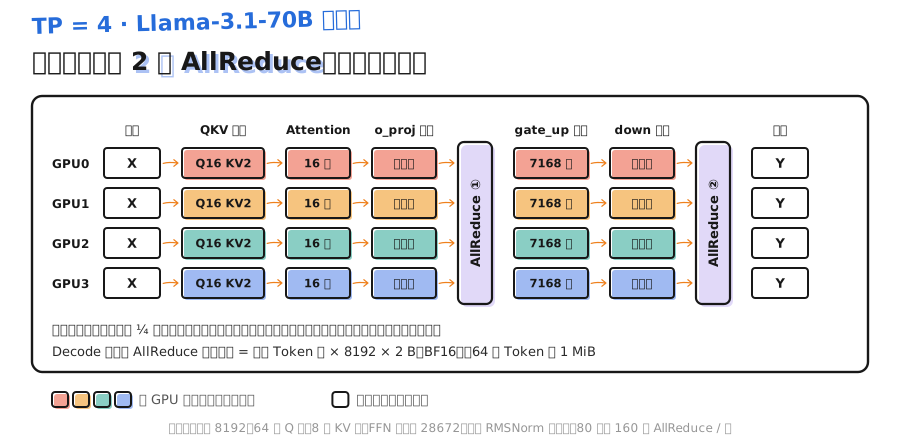
The numbers come from the config: 64 Q heads ÷ 4 = 16, 8 KV heads ÷ 4 = 2, FFN intermediate 28672 ÷ 4 = 7168.
📌 Key point: TP correctness hangs on one fact: after a row split, the partial sums add up to the original result. Every “column + row” pair therefore needs an AllReduce at the end; miss one and the result is wrong.
2. Attention by heads: KV-head replication under GQA
2.1 Head count decides which TP values are legal
Attention is split by head, so Q head count must be divisible by TP size. Llama-3.1-70B has 64 Q heads, so TP can be 1, 2, 4, 8, 16…; Qwen3-32B also has 64 Q heads, same story. In practice TP is also capped by GPUs per node; common values are 2, 4, 8.
2.2 When there are fewer KV heads than TP
GQA lets several Q heads share one K/V group. Llama-3.1-70B has only 8 KV heads; at TP=16 a card does not get a full KV head. vLLM’s fix is replication: when TP exceeds KV head count, each card stores 1 KV head, and each KV head is copied onto TP / KV-heads cards (TP must then be divisible by KV head count).
The figure compares TP=8 and TP=16; blue cells are Q heads per card, green cells are which KV head that card stores:
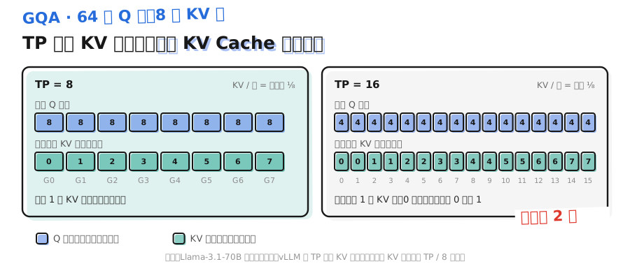
Consequences of replication:
- Per-card KV Cache no longer shrinks with TP. Raising TP from 8 to 16 halves weights per card, but KV per token stays the same. In section 6.1’s estimate, TP=16 KV capacity is only about 18% above TP=8.
- Total KV memory doubles. The same KV lives on two cards; across 16 cards the KV total is 2× the no-replication case.
So for GQA models, KV head count is TP’s natural ceiling. Beyond that, scale further with PP or DP. vLLM also offers Decode Context Parallel (DCP), which shards KV Cache along the token dimension to remove this duplication; section 6.6 covers it.
⚠️ Note: MLA (e.g. DeepSeek-V3) caches one compressed latent vector and has no “KV heads” to split; under TP every card must store the full latent KV. That is one reason DeepSeek-V3-class models usually put attention on DP rather than a large TP (section 6.4).
3. Communication ledger: how long two AllReduces take
3.1 Cost of one AllReduce
nccl-tests performance docs derive AllReduce transfer time: size- data on cards needs transfers per element, shared across links of bandwidth , so ideal time is . Add fixed overhead and total time is about:
is per-card link bandwidth; is fixed cost (kernel launch, alignment, link latency). The first term does not depend on data size; the second scales with it.
3.2 Decode messages are tiny
In Decode, , with the token count this step. Llama-3.1-70B (, BF16):
| 📊 Tokens this step | per AllReduce | Bandwidth term at TP=8 (450 GB/s) |
|---|---|---|
| 1 | 16 KiB | About 0.06 µs |
| 64 | 1 MiB | About 4 µs |
| 8192 (one Prefill chunk) | 128 MiB | About 520 µs |
In Decode the bandwidth term is only a few microseconds—same order as fixed overhead or smaller—so TP communication in Decode is latency-bound. 160 AllReduces per step at +10 µs each adds 1.6 ms to TPOT.
Prefill handles thousands of tokens at once; messages grow to hundreds of MiB and become bandwidth-bound, where NVLink vs PCIe gaps widen several times.
💡 Tip: Sweep message sizes from 8 B to hundreds of MiB with nccl-tests all_reduce_perf on your machine to see the latency/bandwidth boundary. Reported busbw already multiplies by , so you can compare it directly to link bandwidth.
4. Why TP stays inside a node
On an 8-GPU H100 SXM server, GPUs are fully connected through NVLink and NVSwitch; NVIDIA quotes 900 GB/s NVLink per card (both directions). Cross-node traffic goes through NICs: on a DGX B200, 8 GPUs pair with 8 single-port ConnectX-7 at 400 Gb/s each, about 50 GB/s per GPU on average.
| 📊 Link | Per-card bandwidth (one direction) | Relative to NVLink 4 |
|---|---|---|
| NVLink 4 (H100) | 450 GB/s | 1× |
| PCIe Gen5 x16 | 64 GB/s | About 1/7 |
| InfiniBand NDR 400 Gb/s | 50 GB/s | About 1/9 |
Spread TP=16 across two 8-GPU machines and every AllReduce must cross NICs. Under Ring, the whole ring is gated by the slowest hop: bandwidth drops from 450 GB/s to 50 GB/s, and cross-machine latency is higher than in-node. Two calls per layer, hundreds per step—the cost stacks up fast.
Left in the figure: TP=16 spanning two machines. Right: TP=8 stays in-node, PP=2 links the two machines:
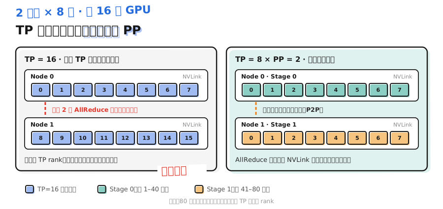
That is the vLLM docs’ advice: TP size = GPUs per node, PP size = node count. PP sends activations once per stage boundary each step; call count drops from hundreds to single digits.
The exception is rack-scale NVLink systems such as GB200 NVL72, where 72 GPUs share one NVLink domain. There the “node” boundary changes; TP can cross physical servers, and the criterion becomes “same NVLink domain or not.”
5. TP degree: separate latency from throughput
Raising TP does several things at once:
- Less weight read per card: Decode memory time per step drops about —the main latency win.
- Call count unchanged, more cards per call: still AllReduces per step; fixed overhead does not fall with and takes a larger share of total time.
- Smaller matrices per card: GEMM’s N or K is cut to ; small matrices struggle to fill Tensor Cores, especially in Prefill.
- More free memory per card: weights and KV (within KV head count) shrink by , so more concurrent requests fit.
The first three say doubling TP does not cut latency in half, and per-card throughput often falls. The fourth says that when KV capacity is the bottleneck, larger TP lets each card serve more requests and per-card throughput can rise.
Pope et al.’s PaLM inference work reached a similar conclusion: no sharding layout is best at every batch size; low latency and high throughput want different layouts. For vLLM deploys:
| 🎯 Goal | TP degree | Notes |
|---|---|---|
| Lowest TPOT (interactive, low concurrency) | As large as the NVLink domain allows, not past KV head count | Latency win from less weight read per card |
| Highest throughput (offline batch) | Smallest TP that fits weights and KV; remaining GPUs as DP | Less sync, larger matrices, higher per-card efficiency |
| In between | Measure a few mixes; compare throughput under the SLO | Same 8 GPUs: TP=8 × 1 replica, TP=4 × 2, TP=2 × 4 |
⚠️ Note: When comparing throughput across TP degrees, normalize by GPU count and compare under the same latency constraint. Higher single-replica throughput at TP=8 than TP=4 does not mean one TP=8 on 8 GPUs beats two TP=4 replicas.
6. TP implementation details in vLLM
6.1 How to launch
One flag on a single node:
vllm serve meta-llama/Llama-3.1-70B-Instruct --tensor-parallel-size 4
vLLM starts one Worker process per GPU. On one node it defaults to Python multiprocessing (mp) to manage Workers; multi-node can use Ray (section 6.5). Workers talk with NCCL collectives.
6.2 Which layers are split
| 📊 Layer | Split | Communication at the end |
|---|---|---|
| Vocab Embedding | By vocab; each card looks up its slice | AllReduce |
| QKV projection | Column-split by head; replicate when KV heads run out | None |
o_proj | Row-split | AllReduce |
gate_up_proj | Column-split | None |
down_proj | Row-split | AllReduce |
| LM Head | Column-split by vocab | Gather logits from all cards, then sample |
| RMSNorm | Not split; one copy per card | None |
Embedding and LM Head vocabs are large (Llama-3.1 is 128256); vocab sharding saves meaningful memory. Section 3.3 covered the matching VocabParallelEmbedding and ParallelLMHead in nano-vllm.
6.3 Custom AllReduce
NCCL’s general algorithms target many topologies and are not the fastest for small in-node messages. vLLM ships its own AllReduce kernel: when in-node GPUs can read each other’s memory directly, cards sum from each other’s buffers and skip several ring hops—friendlier for latency-bound Decode messages. When conditions fail or messages are large, it falls back to NCCL.
If you hit related errors (for example P2P unavailable in some virtualized environments), --disable-custom-all-reduce turns it off so every AllReduce goes through NCCL, which helps isolate the issue.
💡 Tip: When Custom AllReduce is not enabled, the startup log prints why—P2P probe failed, or more than two GPUs linked only by PCIe. If TP performance looks wrong, start with that log line.
7. Hands-on: a rough model of TP degree vs time per token
Below is a hypothetical cost model: only Decode step weight read, KV read, and TP communication; compute, kernel launch, and scheduling are ignored. µs is assumed and matches no measurement. At TP=1 and TP=2 a 70B model does not actually fit; the numbers are only for trend.
# Hypothetical cost model: estimate Decode step memory time and TP communication only;
# ignore compute and kernel launch
HBM = 3.35e12          # H100 SXM memory bandwidth, B/s
NVLINK = 450e9         # NVLink 4 unidirectional, B/s (900 GB/s is bidirectional total)
ALPHA = 10e-6          # fixed cost per AllReduce, assumed
LAYERS, HIDDEN = 80, 8192
WEIGHT_BYTES = 70.6e9 * 2
KV_PER_TOKEN = 320 * 1024        # whole-model KV per token, B
CTX = 4096                        # average context length per request


def step_ms(tp, batch):
    weight = WEIGHT_BYTES / tp / HBM
    kv = batch * CTX * KV_PER_TOKEN / min(tp, 8) / HBM   # KV stops shrinking after TP>8
    msg = batch * HIDDEN * 2
    comm = 0 if tp == 1 else 2 * LAYERS * (ALPHA + 2 * (tp - 1) / tp * msg / NVLINK)
    return (weight + kv + comm) * 1e3, comm * 1e3


print(f"{'TP':>3} {'batch':>5} {'step ms':>8} {'comm':>8} {'Token/s':>9} {'Token/s/GPU':>10}")
for batch in [1, 64]:
    for tp in [1, 2, 4, 8]:
        t, c = step_ms(tp, batch)
        print(f"{tp:>3} {batch:>5} {t:>8.2f} {c:>8.2f} {batch / t * 1e3:>9.0f} {batch / t * 1e3 / tp:>10.0f}")
Output:
 TP batch    step ms      comm   Token/s  Token/s/GPU
  1     1    42.55     0.00        24         24
  2     1    22.88     1.61        44         22
  4     1    12.25     1.61        82         20
  8     1     6.93     1.61       144         18
  1    64    67.79     0.00       944        944
  2    64    35.87     1.97      1784        892
  4    64    19.11     2.16      3350        837
  8    64    10.73     2.25      5967        746
Under these assumptions:
- TP 1 → 8 cuts single-request step time from 42.6 ms to 6.9 ms, about 6.1×, not 8×. The gap is 1.6 ms of communication that does not shrink with TP.
- At batch=64, TP=8 per-card throughput is about 16% below TP=2. If KV capacity is not the bottleneck, four TP=2 replicas on the same 8 GPUs yield higher total throughput.
- Set
ALPHAto 30 µs and re-check TP=8 to feel why TP across nodes or without NVLink is a bad deal.
Real systems also have compute time, Attention kernel efficiency differences, and scheduling. Use the model only for trends; deploy decisions should follow vllm bench serve measurements (section 6.6).
📝 Summary
- TP pairs column and row splits; intermediate activations stay on each card; 2 AllReduces per layer → 160 per step on an 80-layer model.
- Attention is split by head; Q head count must divide by TP; once GQA TP exceeds KV heads, vLLM replicates KV heads and per-card KV stops shrinking.
- Decode AllReduce messages are KiB–MiB and latency-bound; Prefill messages are large and bandwidth-bound.
- NVLink 4 is 450 GB/s one way; a cross-node 400 Gb/s NIC is about 50 GB/s, so keep TP in-node and use PP across nodes.
- Larger TP lowers latency but usually lowers per-card throughput; the opposite can hold when KV capacity is the bottleneck—compare after normalizing by GPU count.
- vLLM’s Custom AllReduce speeds small in-node messages; use
--disable-custom-all-reducewhen debugging.
🎯 Self-check list
- Can derive why FFN column + row equals the original result, and where AllReduce sits
- Can judge legal TP degrees from Q and KV head counts, and from which TP KV-head replication starts
- Can estimate one AllReduce with and tell latency- vs bandwidth-bound
- Can compare per-card bandwidth of NVLink, PCIe, and InfiniBand and explain why TP stays in-node
- Can explain why doubling TP does not halve latency and why per-card throughput may fall
- Can pick TP degree and replica count for “lowest latency” vs “highest throughput”
- Can name which vLLM layers are vocab-split and what
--disable-custom-all-reduceis for
📚 References
- Megatron-LM: Training Multi-Billion Parameter Language Models Using Model Parallelism
- Efficiently Scaling Transformer Inference
- NVIDIA H100 Tensor Core GPU
- NVIDIA NVLink and NVLink Switch
- NVIDIA DGX B200 User Guide
- nccl-tests Performance (AllReduce timing model and busbw)
- vLLM docs: Parallelism and Scaling
- vLLM source: vllm/model_executor/layers/linear.py (v0.32.0)
- vLLM source: vllm/distributed/device_communicators/custom_all_reduce.py (v0.32.0)