3.3 Model skeleton and core operators
Layer by layer through nano-vllm's Qwen3: RMSNorm, RoPE, SwiGLU, parallel Linear and tensor-parallel sharding, vocab-parallel Embedding/LMHead, Attention's KV write and two FlashAttention paths, and the Sampler's temperature sampling
📑 Contents
- 1. Start from one Qwen3 layer
- 2. RMSNorm: a cheaper normalization
- 3. RoPE: rotary position embedding
- 4. SwiGLU: SiluAndMul
- 5. The parallel Linear family and tensor parallelism
- 6. Vocab-parallel Embedding and LMHead
- 7. Attention: writing KV and two paths
- 8. Assembling Qwen3
- 9. Sampler: from logits to a token
- Summary
- Self-check checklist
- References
1. Start from one Qwen3 layer
What the execution layer finally runs is the Transformer in models/qwen3.py. Start with the shape of one Qwen3DecoderLayer; that sets the call order of the operators.
Qwen3 uses a Pre-Norm + residual structure: normalization sits before each sublayer, and the residual skips over the sublayer. nano-vllm folds the residual add into the norm itself:
class Qwen3DecoderLayer(nn.Module):
    def forward(self, positions, hidden_states, residual):
        if residual is None:                       # First layer: residual starts from the input
            hidden_states, residual = self.input_layernorm(hidden_states), hidden_states
        else:                                       # Later layers: norm also emits the new residual
            hidden_states, residual = self.input_layernorm(hidden_states, residual)
        hidden_states = self.self_attn(positions, hidden_states)
        hidden_states, residual = self.post_attention_layernorm(hidden_states, residual)
        hidden_states = self.mlp(hidden_states)
        return hidden_states, residual
Each layer does two things: normalize + attention first, then normalize + MLP. The residual residual is threaded from the first layer all the way to the last. RMSNorm can take the previous residual, add it in, normalize, and return the new residual after the add, so the DecoderLayer does not have to keep writing x = x + sublayer(norm(x)). The sections below unpack each operator this layer uses.
2. RMSNorm: a cheaper normalization
LLMs commonly replace LayerNorm with RMSNorm. It drops the mean subtraction and the bias, and only scales by the root-mean-square—less compute, similar quality:
nano-vllm’s RMSNorm has two entry points, both with @torch.compile. Plain normalization:
@torch.compile
def rms_forward(self, x):
    orig_dtype = x.dtype
    x = x.float()                                  # Upcast to fp32 for the variance
    var = x.pow(2).mean(dim=-1, keepdim=True)
    x.mul_(torch.rsqrt(var + self.eps))
    return x.to(orig_dtype).mul_(self.weight)      # Cast back, then multiply by γ
The residual-add version first adds the residual in fp32, casts the sum back to the original dtype as the new residual, then normalizes the sum:
@torch.compile
def add_rms_forward(self, x, residual):
    orig_dtype = x.dtype
    x = x.float().add_(residual.float())           # Residual add
    residual = x.to(orig_dtype)                    # New residual = value after the add
    var = x.pow(2).mean(dim=-1, keepdim=True)
    x.mul_(torch.rsqrt(var + self.eps))
    return x.to(orig_dtype).mul_(self.weight), residual
💡 Tip: the previous section’s hidden_states, residual = self.input_layernorm(hidden_states, residual) calls this version. Residual add and normalization live in the same torch.compile function, so the compiler can fuse them into fewer kernels. The variance is computed in fp32 to avoid losing precision when squaring and summing in bf16.
3. RoPE: rotary position embedding
RoPE (Rotary Position Embedding) does not add a position vector to the input. Instead it rotates each pair of Q and K dimensions by an angle that depends on position, so the Q·K dot product depends only on relative position. The frequency table is precomputed at init; cos and sin are concatenated into one buffer:
inv_freq = 1.0 / (base ** (torch.arange(0, rotary_dim, 2).float() / rotary_dim))
t = torch.arange(max_position_embeddings).float()
freqs = torch.einsum("i,j->ij", t, inv_freq)            # [position, rotary_dim/2]
cache = torch.cat((freqs.cos(), freqs.sin()), dim=-1)   # [position, rotary_dim]
self.register_buffer("cos_sin_cache", cache.unsqueeze_(1), persistent=False)  # Extra mid dim to align with the head dim
At forward time the last dimension is split into front and back halves as ; dimension pairs with for a 2D rotation:
@torch.compile
def forward(self, positions, query, key):
    cos, sin = self.cos_sin_cache[positions].chunk(2, dim=-1)  # Lookup by position
    query = apply_rotary_emb(query, cos, sin)    # Internally chunk into halves and rotate as above
    key = apply_rotary_emb(key, cos, sin)
    return query, key
A few things to watch:
- 🔑 RoPE acts only on Q and K, never on V. Position only needs to show up in the attention scores; V is the content being weighted and summed.
- 🔑
forwardcarries@torch.compile. RoPE is a small elementwise op; after compile it can fuse into a few kernels and cut memory traffic. nano-vllm usestorch.compileon the elementwise ops RMSNorm, RoPE, SiluAndMul, and Sampler. get_ropehas@lru_cache(1); identical parameters return the same object, so all 28 layers share onecos_sin_cacheinstead of storing a table per layer.- Even when the config has
rope_scaling, the code only readsrope_thetafrom it; NTK / YaRN and other length-extrapolation logic is not implemented.
4. SwiGLU: SiluAndMul
Qwen3’s FFN uses the SwiGLU activation. It projects the input into two parts: one goes through SiLU as a «gate», the other is «data», then the two are multiplied elementwise:
nano-vllm splits that into two pieces: the projection is one MergedColumnParallelLinear that produces gate and up in one shot (output dim is 2× the intermediate dim), and the activation is a short SiluAndMul:
class SiluAndMul(nn.Module):
    @torch.compile
    def forward(self, x):
        gate, up = x.chunk(2, dim=-1)      # Front half is gate, back half is up
        return F.silu(gate) * up
💡 Tip: merging gate and up into one Linear then splitting uses the GPU better than two small matmuls: x is read once, and kernel launches are halved. Merging QKV into qkv_proj is the same idea.
5. The parallel Linear family and tensor parallelism
Tensor Parallelism (TP) splits one large matmul across multiple GPUs. nano-vllm’s linear.py wraps that mechanism as a family of Linear subclasses; pick the right type in the model code and you get TP. The key is which dimension you shard on. The figure below uses TP=2: blue and yellow are the shards owned by rank0 and rank1; red is the only all_reduce that needs communication:
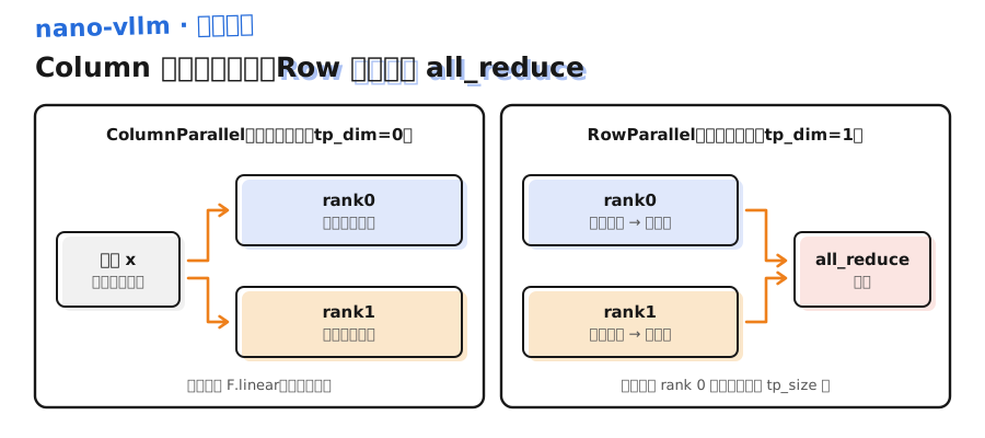
ColumnParallelLinear(tp_dim=0): shards along the output dim; each GPU computes a slice of output columns. Weight loading usesnarrowalong dim 0 for this rank’s shard; forward is plainF.linearand needs no communication.RowParallelLinear(tp_dim=1): shards along the input dim; each GPU takes part of the input and forms a partial sum. So when TP>1 the forward ends withdist.all_reduce(y)to add the results; bias is added only on rank 0 so it is not accumulatedtp_sizetimes.QKVParallelLinear(subclass of ColumnParallel): merges the Q, K, V projections into one large matrix; output dim is(num_heads + 2 * num_kv_heads) * head_dim. Weight loading locates each segment’s offset by the stringshard_id("q"/"k"/"v").MergedColumnParallelLinear(subclass of ColumnParallel): merges gate and up (used by SwiGLU above); weight loading indexesoutput_sizesby the integershard_id(0=gate, 1=up).
Laid out along the Transformer data path, Column and Row appear in pairs:
| Position | What to use | Why |
|---|---|---|
| QKV projection | QKVParallelLinear (Column) | Shard by head; each GPU computes the heads it owns |
Attention output projection o_proj | RowParallelLinear | Gather the heads back; needs all_reduce |
FFN first layer gate_up | MergedColumnParallelLinear (Column) | Shard the intermediate dim |
FFN second layer down | RowParallelLinear | Pull the intermediate dim back; needs all_reduce |
📌 Key point: Column shards the output, Row gathers the input. They pair front-to-back; activations stay sharded inside each GPU with no communication in between, and only one all_reduce runs at the end of each sublayer. So each Transformer layer has exactly 2 all_reduces (one for Attention’s o_proj, one for FFN’s down_proj). That is the Megatron-LM TP sharding pattern; nano-vllm’s linear.py implements it in 156 lines.
⚠️ Note: QKV is sharded by head, so Qwen3Attention asserts that both the number of attention heads and the number of KV heads are divisible by tp_size. Qwen3-0.6B has 16 Q heads and 8 KV heads, so the TP degree can only be 1, 2, 4, or 8. In nano-vllm the number of KV heads is also the upper bound on TP for a GQA model (vLLM will replicate KV heads when TP exceeds the KV-head count; nano-vllm does not).
6. Vocab-parallel Embedding and LMHead
Qwen3’s vocabulary is about 150k rows. Embedding and LMHead weights are large too, so they are also sharded. nano-vllm makes them vocab-parallel: each GPU holds one slice of the vocabulary.
VocabParallelEmbedding.forward has to handle «this token is not on my GPU»:
def forward(self, x):
    if self.tp_size > 1:
        mask = (x >= self.vocab_start_idx) & (x < self.vocab_end_idx)  # Tokens this GPU owns
        x = mask * (x - self.vocab_start_idx)   # Shift to local indices; out-of-range become 0 for now
    y = F.embedding(x, self.weight)
    if self.tp_size > 1:
        y = mask.unsqueeze(1) * y               # Zero rows that are not this GPU's
        dist.all_reduce(y)                      # Sum: only one GPU has a non-zero vector per token
    return y
Every GPU looks up the table, but only the GPU that owns that token produces a non-zero vector; the others output 0. After all_reduce the sum is the full result. With TP=1 both if blocks are skipped and it degenerates to plain F.embedding.
ParallelLMHead is its subclass and projects hidden states to vocabulary logits. Two details:
def forward(self, x):
    context = get_context()
    if context.is_prefill:
        last_indices = context.cu_seqlens_q[1:] - 1   # Last position of each sequence
        x = x[last_indices].contiguous()               # Keep only the last token
    logits = F.linear(x, self.weight)
    if self.tp_size > 1:
        # Each GPU computes one slice of the vocab; gather to rank0 then concat into full logits
        all_logits = [...] if self.tp_rank == 0 else None
        dist.gather(logits, all_logits, 0)
        logits = torch.cat(all_logits, -1) if self.tp_rank == 0 else None
    return logits
- 🔑 Prefill only takes the last token: generating the next token only needs logits at the last position of each sequence.
cu_seqlens_q[1:] - 1finds that last index in the packed tensor, so the whole prompt is not projected to vocab dim. For a 1000-token prompt, LMHead only projects 1 row, not 1000. - 🔑 LMHead uses
gather, notall_reduce: the vocabulary is sharded on the output dim (each GPU computes different logit columns); you need concatenation, not a sum, sodist.gathercollects onto rank 0 and thencat, while other ranks returnNone. Embedding lookup is equivalent to a one-hot times the weight matrix, and the vocabulary is the input dim of that multiply, so it usesall_reduce. Shard the input dim → reduce; shard the output dim → gather, the same Column/Row rule as in section 5.
7. Attention: writing KV and two paths
attention.py does two things: first write the newly computed K/V into the KV Cache, then run the attention compute. Prefill and decode call different FlashAttention interfaces for that compute.
7.1 Writing K/V into the Cache with Triton
Each token’s K/V must land in the matching slot of the KV Cache. Slot ids come from the slot_mapping computed upstream (see 3.6); here we only write by id. nano-vllm does that with a short Triton kernel:
@triton.jit
def store_kvcache_kernel(key_ptr, key_stride, value_ptr, value_stride,
                         k_cache_ptr, v_cache_ptr, slot_mapping_ptr, D: tl.constexpr):
    idx = tl.program_id(0)                 # Each program handles one token
    slot = tl.load(slot_mapping_ptr + idx)
    if slot == -1:                         # -1 means this token need not be written (padding)
        return
    # Use the passed strides to locate the D elements of token idx; write to that cache slot row
    key = tl.load(key_ptr + idx * key_stride + tl.arange(0, D))
    value = tl.load(value_ptr + idx * value_stride + tl.arange(0, D))
    cache_offsets = slot * D + tl.arange(0, D)
    tl.store(k_cache_ptr + cache_offsets, key)
    tl.store(v_cache_ptr + cache_offsets, value)
The wrapper store_kvcache pulls (N, num_heads, head_dim) from key.shape and sets D = num_heads * head_dim. The incoming key is a KV-head tensor, so num_heads here is really this rank’s KV-head count, and D is the length of one token’s K (or V) vector in one layer. key_stride / value_stride are passed from outside as key.stride(0); the wrapper also asserts key.stride(-1) == 1, key.stride(1) == head_dim, and k_cache.stride(1) == D, so each token’s D elements are contiguous in memory and the kernel can read/write a whole segment in one go.
💡 Tip: the same logic in PyTorch is roughly k_cache.view(-1, D)[slot_mapping] = key.view(N, D). The problem is positions where slot == -1: when a CUDA Graph replays, the decode batch is padded to a fixed size, and padded tokens get slot -1 (covered in 3.6)—those positions must not be written. In PyTorch you would mask them out first; the filtered length then varies with the data and does not fit a CUDA Graph. The Triton kernel handles one token per program, returns immediately on -1, keeps tensor shapes fixed, and can be captured by a Graph.
7.2 Two paths: prefill uses varlen, decode uses with_kvcache
Attention.forward first calls store_kvcache to write the cache, then branches on context.is_prefill:
def forward(self, q, k, v):
    context = get_context()
    k_cache, v_cache = self.k_cache, self.v_cache
    if k_cache.numel() and v_cache.numel():    # Only write once the cache is allocated
        store_kvcache(k, v, k_cache, v_cache, context.slot_mapping)
    if context.is_prefill:
        if context.block_tables is not None:   # Historical KV present: read from the full cache
            k, v = k_cache, v_cache
        o = flash_attn_varlen_func(
            q, k, v,
            cu_seqlens_q=context.cu_seqlens_q, cu_seqlens_k=context.cu_seqlens_k,
            max_seqlen_q=context.max_seqlen_q, max_seqlen_k=context.max_seqlen_k,
            softmax_scale=self.scale, causal=True,
            block_table=context.block_tables)
    else:                                       # decode
        o = flash_attn_with_kvcache(
            q.unsqueeze(1), k_cache, v_cache,
            cache_seqlens=context.context_lens, block_table=context.block_tables,
            softmax_scale=self.scale, causal=True)
    return o
The two paths match the two phases:
- 🔑 Prefill uses
flash_attn_varlen_func: one call computes attention over the whole prompt; several variable-length sequences are packed together and split by the two cumulative-length arrayscu_seqlens_q/cu_seqlens_k;causal=Truekeeps each position looking only at the past. If some of this step’s K/V already sits in the Cache,ModelRunnerpassesblock_tables; thenk, vare replaced by the fullk_cache/v_cacheand the kernel reads the complete historical K/V from physical blocks viablock_table. Two cases trigger that: a prefix-cache hit, or a later chunk of chunked prefill (earlier chunks were written to the Cache on the previous step). In both cases Q is shorter than K; the shared condition iscu_seqlens_k[-1] > cu_seqlens_q[-1]. - 🔑 Decode uses
flash_attn_with_kvcache: each sequence adds only one token (q.unsqueeze(1)inserts the length dim of 1); all K/V come from the Cache;cache_seqlenstells the kernel how long each sequence currently is;block_tabletells it which physical blocks to read. - The scale is
scale = head_dim ** -0.5, i.e. the usual .
📌 Key point: «Prefill is compute-bound, Decode is memory-bound» shows up in code as the two phases calling different FlashAttention interfaces. How KV Cache physical blocks are assigned and how slots are computed is left to 3.4 and 3.6; here it is enough that Attention both writes and reads the Cache.
8. Assembling Qwen3
With those operators in hand, models/qwen3.py wires them into Qwen3’s structure. Compared with a LLaMA-style implementation there are two differences.
① After the QKV projection, per-head RMSNorm on Q and K. Qwen3 adds an RMSNorm on each attention head’s Q and K (QK-Norm) to stabilize training:
def forward(self, positions, hidden_states):
    qkv = self.qkv_proj(hidden_states)
    q, k, v = qkv.split([self.q_size, self.kv_size, self.kv_size], dim=-1)
    q = q.view(-1, self.num_heads, self.head_dim)     # Reshape to [token, head, head_dim]
    k = k.view(-1, self.num_kv_heads, self.head_dim)
    v = v.view(-1, self.num_kv_heads, self.head_dim)
    if not self.qkv_bias:                             # Qwen3 takes this branch
        q = self.q_norm(q)                            # Normalize per head along head_dim
        k = self.k_norm(k)
    q, k = self.rotary_emb(positions, q, k)           # Then apply rotary positions
    o = self.attn(q, k, v)
    return self.o_proj(o.flatten(1, -1))              # Flatten the head dim, project back to hidden
🔑 Core idea: RMSNorm acts on the last dim head_dim, so reshaping to [token, head, head_dim] and feeding it in is per-head normalization. QK-Norm is enabled only when not self.qkv_bias. qkv_bias comes from the HF config’s attention_bias (default treated as True); in Qwen3’s config it is false, so the QK-Norm branch runs. Qwen2-style structures with QKV bias skip QK-Norm.
② Weight mapping packed_modules_mapping. nano-vllm merges q/k/v into qkv_proj and gate/up into gate_up_proj, while the HuggingFace checkpoint still has five separate weights. At load time loader.py walks safetensors weight names, substring-matches this table, and translates the original name into the merged parameter name plus shard_id:
packed_modules_mapping = {
    "q_proj":    ("qkv_proj", "q"),      # String shard_id
    "k_proj":    ("qkv_proj", "k"),
    "v_proj":    ("qkv_proj", "v"),
    "gate_proj": ("gate_up_proj", 0),    # Integer shard_id
    "up_proj":   ("gate_up_proj", 1),
}
Section 5’s «QKV uses string shard_id, Merged uses integer shard_id» comes from this table: the two classes’ weight_loaders each handle one of the value types.
Two more engineering details:
tie_word_embeddings: small models such as Qwen3-0.6B share one weight table between Embedding and LMHead. InQwen3ForCausalLM.__init__,self.lm_head.weight.data = self.model.embed_tokens.weight.datamakes both parameters point at the same storage; loading the embed weights then fills lm_head as well, using only one copy of GPU memory.compute_logitscalls LMHead separately:forwardstops at the hidden state; logits are computed bycompute_logitson its own. That way a CUDA Graph only needs to capture through the hidden state; LMHead’s «prefill takes only the last token» logic and the sampling that follows stay outside the Graph.
9. Sampler: from logits to a token
Once rank 0 has the logits, Sampler samples the next token with each sequence’s own temperature. The whole class is one @torch.compile forward:
class Sampler(nn.Module):
    @torch.compile
    def forward(self, logits, temperatures):
        logits = logits.float().div_(temperatures.unsqueeze(dim=1))  # Divide each row by its temperature
        probs = torch.softmax(logits, dim=-1)
        noise = torch.empty_like(probs).exponential_(1).clamp_min_(1e-10)  # E ~ Exp(1)
        return probs.div_(noise).argmax(dim=-1)                       # argmax(p / E)
The last line does not call torch.multinomial; it divides each probability by an independent exponential random number and takes the max. That is an equivalent form of the Gumbel-max trick; the claim is:
A short derivation: the max of is the same as the min of , and is exponential with rate . Among a set of independent exponential random variables, the probability that the -th arrives first is , which is exactly sampling from .
- 🔑 Same effect as
multinomial, but all elementwise ops plus one argmax: the division, exponential noise, and argmax can all be fused bytorch.compile; you do not needmultinomial’s prefix-sum-then-binary-search path. - 🔑 Temperature only scales the logits: higher temperature flattens the softmax and increases randomness. Temperature 0 would divide by 0 on the first line—that is why
SamplingParamsassertstemperature > 1e-10at the entry point (see 3.2). - Sampling runs only on rank 0. In
ModelRunner.runonly rank 0 callsprepare_sampleandsampler; other ranks’compute_logitsreturnsNone, and so doesrun. - nano-vllm does not implement top-k, top-p, repetition penalty, and so on;
SamplingParamsalso has only three fields.
📝 Summary
Qwen3DecoderLayeris Pre-Norm + residual; nano-vllm folds the residual add intoRMSNorm, so the backbone only threads oneresidual.- RMSNorm drops mean subtraction and only scales by RMS, with variance in fp32; RoPE rotates Q/K in front/back half pairs and never touches V; 28 layers share one
cos_sin_cache; SwiGLU isMergedColumnParallelLinear+SiluAndMul. These elementwise ops all use@torch.compilefor fusion. - The parallel Linear family follows «Column shards the output, Row gathers the input»; each Transformer layer has exactly 2
all_reduces (o_projanddown_proj); the TP degree must divide both the Q-head count and the KV-head count. - In vocab parallelism, Embedding uses
all_reduceand LMHead usesgather; during prefill LMHead only projects the last token of each sequence. - Attention first writes K/V into the Cache with a Triton kernel (skipping padding where slot = -1), then branches by phase: prefill goes through
flash_attn_varlen_func, and when historical KV is already in the Cache it also passesblock_table; decode goes throughflash_attn_with_kvcache. - Qwen3’s distinctive pieces are per-head QK-Norm and the
packed_modules_mappingweight-merge map;tie_word_embeddingslets LMHead share storage with Embedding. Samplerimplements temperature sampling asargmax(p / E)withE ~ Exp(1), equivalent to drawing fromsoftmax(logits / T), and runs only on rank 0.
🎯 Self-check checklist
- Can draw the
Qwen3DecoderLayerdata path and explain why the residual can live inside RMSNorm - Can say what RMSNorm saves versus LayerNorm, and why RoPE only acts on Q/K
- Can explain why SwiGLU merges gate and up into one Linear then splits
- Can tell ColumnParallelLinear from RowParallelLinear by shard dim and communication, and say why each layer has exactly 2 all_reduces
- Can name the TP degrees usable for Qwen3-0.6B in nano-vllm, and where the limit comes from
- Can explain why vocab-parallel Embedding uses
all_reducewhile LMHead usesgather - Can name which FlashAttention function Attention calls in prefill vs decode, and when prefill also passes
block_table - Can explain why
store_kvcacheis written in Triton rather than with PyTorch index assignment - Can prove that
argmax(p / E)(E ~ Exp(1)) is equivalent to sampling from probabilityp
📚 References
- nano-vllm GitHub repository
- Qwen3 Technical Report (Qwen Team, 2025)
- Qwen3-0.6B model card
- RoFormer: Enhanced Transformer with Rotary Position Embedding (Su et al., 2021)
- Root Mean Square Layer Normalization (Zhang & Sennrich, 2019)
- GLU Variants Improve Transformer (Shazeer, 2020)
- Megatron-LM: Training Multi-Billion Parameter Language Models Using Model Parallelism (Shoeybi et al., 2019)
- FlashAttention: Fast and Memory-Efficient Exact Attention with IO-Awareness (Dao et al., 2022)
- FlashAttention interface docs (flash_attn_interface.py)
- Triton documentation