4.1 Quantization basics
Understand quantization and dequantization through a ruler with limited ticks: Scale, zero-point, bit width, granularity, calibration, and the difference between PTQ and QAT
Quantization is like switching to a ruler with fewer tick marks: you used to read millimeters, now you only get centimeters. The data gets smaller, and the readings get coarser. Quantization answers three questions: how you set the ticks (Scale and zero-point), how many values share one ruler (granularity), and how you keep the model from suffering too much from the rounding error (calibration and PTQ/QAT).
This section sticks to framework-agnostic basics. SmoothQuant, GPTQ/AWQ, KV Cache quantization, and low-bit floating point in later sections all build on these ideas.
⏰ Freshness note: This section covers general principles and does not depend on a specific framework version. Rounding rules follow the ONNX QuantizeLinear operator definition.
📑 Contents
- 1. First, separate what you are quantizing
- 2. Value mapping, Scale, and Zero-point
- 3. Tensor axes and quantization granularity
- 4. Calibration: picking the range for the ruler
- 5. PTQ and QAT
- 6. Hands-on: watching outliers hurt
- Summary
- Self-check list
- References
1. First, separate what you are quantizing
At inference time, GPU memory mostly holds three kinds of data. All three can be quantized, but they behave differently:
| 📊 Object | What the data looks like | Main win after quantization |
|---|---|---|
| Weight | Fixed after training; you can process it offline at leisure | Smaller model; less weight traffic per step |
| Activation | Changes with every input; must be handled online | Lets matrix multiplies use low-precision kernels |
| KV Cache | Grows with requests and context | Less cache per historical token |
The common notation W4A16 means 4-bit weights and 16-bit activations; W8A8 means both are 8-bit. That notation only describes the two inputs of linear layers. KV Cache precision has to be stated separately.
A rough back-of-the-envelope: 7B parameters all in 16-bit are about 14 GB of raw data; all in 4-bit about 3.5 GB (decimal GB, ignoring quantization parameters). The data shrinks to a quarter; how much faster you get depends on where the bottleneck sits, as Chapter 1 covered.
2. Value mapping, Scale, and Zero-point
2.1 Quantization and dequantization
FP16 itself only represents finitely many values. Quantization maps those onto even fewer codes. For uniform integer encoding, the usual affine quantization is written:
- is Scale, the numeric gap between two neighboring ticks on the ruler;
- is Zero-point, the integer tick that real-valued 0 lands on;
- Quantization produces the code ; dequantization uses and to turn the code back into an approximate value .
The round rule is up to the implementation. ONNX’s integer QuantizeLinear, for example, uses round half to even.
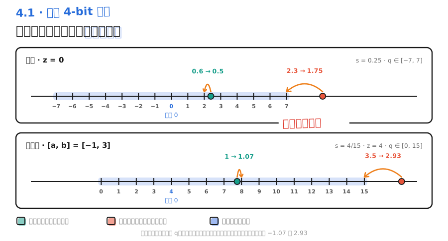
Take : becomes , and reading it back gives . The discarded 0.04 is gone for good. Switch to , and the same 0.26 becomes 4 and reads back as 0.25. So “keep one decimal place” is just the coincidence of . What actually decides which values you can represent is bit width and Scale. Every number in a bucket lands on the same tick; with , 0.251, 0.26, and 0.349 all map to 3.
The figure below draws two 4-bit ranges on the same real axis (symmetric uses ; asymmetric reuses from section 2.3). The blue band is the covered range: green points snap to the nearest tick and create rounding error; red points fall outside the range and get clamped to an endpoint, creating clipping error. Quantization error is basically these two kinds.
2.2 Symmetric quantization
When positive and negative values are roughly balanced, you can set . A common INT8 convention uses only :
The INT8 type itself can represent . Here we deliberately drop it so both ends stay symmetric. 4-bit likewise uses only ; the symmetric axis in the figure above is built that way. The upside is that dequantization is just a multiply by Scale, and matrix multiplies do not need a zero-point correction.
2.3 Asymmetric quantization
If the data all sits in , symmetric quantization wastes half the codes on unused negatives. Asymmetric quantization lets the range hug the data: pick an interval that contains 0, then compute
For example and code range give . At , , and dequantization yields . The zero-point has to be an integer, so the actual range endpoints shift a little.
Asymmetric quantization fits skewed distributions better. The cost is an extra zero-point to store and one more correction at compute time. All-zero tensors need special handling so you do not end up with .
2.4 Bit width sets how dense the ticks are
With a fixed range, every bit you drop halves the number of bins and doubles the bin width. Uniformly quantizing :
| 📊 Bit width | Number of codes | Gap between ticks | Max rounding error |
|---|---|---|---|
| 8-bit | 256 | ||
| 4-bit | 16 | ||
| 2-bit | 4 |
From 8-bit to 4-bit, the gap becomes about 17×. That is why low-bit schemes almost always pair with finer granularity or smarter error compensation. GPTQ, AWQ, and KIVI later on are all about that.
3. Tensor axes and quantization granularity
3.1 Get the matrix axes straight
This chapter consistently uses the math layout :
Rows of are tokens; columns are input channels. PyTorch’s nn.Linear.weight has shape , which is exactly the transpose of here. When you read code, do not swap “row” and “column”.
Look at a tiny activation matrix (3 tokens, 4 channels):
Column 3 is large on every token. That “a few channels stay systematically large” pattern is common in LLM activations, and it is the starting point for SmoothQuant in section 4.2.
3.2 How many values share one ruler
Granularity is “how large a group of values shares one Scale”. Smaller groups fit local data better, but you also store and read more Scales:
| 📊 Granularity | Shared scope | Typical use | Cost |
|---|---|---|---|
| Per-tensor | One Scale for the whole tensor | Static activations, FP8 weights | One outlier hurts everyone |
| Per-channel | One Scale per output channel | INT8 weights | Scale count equals output channel count |
| Per-group | One Scale per consecutive elements (e.g. 128) | INT4 weights | More Scales; the kernel must dequantize by group |
| Per-token | One Scale per token | Dynamic activations | Runtime must find the max of each row first |
The figure below draws the four granularities on the layout. Cells with the same color and label share one Scale. The in the lower right is the matrix above; the red dashed box marks the persistently large third input channel:
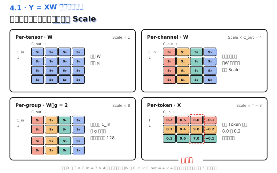
On the above, Per-token gives each row its own range, but 8.0 and 0.2 in the same row still share one ruler, so the small values stay coarse. Granularity can only cut along some axis. If that cut does not line up with where the outliers live, finer groups do not help. Activation outliers sit along channels, while matrix multiplication needs the activation Scale to factor out of the sum (so you can only split by token). That is the root of why W8A8 is hard.
4. Calibration: picking the range for the ruler
4.1 Too wide blurs; too narrow clips
Scale is set by the range. Take the range out to the max and outliers fit, but most of the data crowds into a few bins and rounding error grows. Narrow the range and most values read finer, but anything outside gets clipped. Calibration is finding the balance between rounding error and clipping error. Common approaches include taking the max, taking a percentile, or searching a clip point against MSE or output error.
Weights are fixed, so you can gather stats from the weights themselves. Activations need real samples before you see the distribution; that batch is the calibration set. It should cover the languages, chat templates, and input lengths you see in production, and it must be kept separate from the eval set, or scores look too optimistic.
4.2 Static vs dynamic
- Static quantization: compute Scales offline on the calibration set and use them at inference. Cheapest at runtime, but a shift in input distribution can make them wrong.
- Dynamic quantization: compute Scales online from the current data. Closer to the input; the cost is finding the max every time.
“Dynamic” by itself does not say anything about granularity. When a scheme calls itself dynamic quantization, confirm three things: when Scale is computed, along which axis, and which operators it applies to.
5. PTQ and QAT
PTQ (Post-Training Quantization) quantizes after training is done, at most adjusting Scales or weights with a little calibration data. QAT (Quantization-Aware Training) makes the model forward with quantization error during training or fine-tuning, so the parameters adapt to it.
QAT’s forward pass uses Fake Quant: quantize, then immediately dequantize. The data stays floating point, but it already carries rounding error. The derivative of round is almost everywhere 0, so backprop uses the STE (Straight-Through Estimator) approximation: pass gradients through unchanged inside the range, and usually zero them outside.
| 📊 Dimension | PTQ | QAT |
|---|---|---|
| What you need | A trained model plus a little calibration data | Training pipeline, data, and compute |
| How you control error | Pick Scale and clip points, or do layer-wise compensation (GPTQ/AWQ) | Let parameters adapt to quantization during training |
| When it fits | 8-bit, 4-bit weights, and other settings where error stays manageable | Lower bit widths, or when PTQ accuracy is not good enough |
| Still need to verify | Accuracy on the target task | Accuracy on the target task, and whether the inference kernel supports the format |
LLM inference deployment is mostly PTQ. The methods later in this chapter are basically all PTQ.
💡 Tip: PTQ does not mean “no data”. Most methods still need a calibration set. QAT is also not training in integers; the main compute stays floating point, and quantization error is simulated with Fake Quant.
6. Hands-on: watching outliers hurt
The pure-Python snippet below does symmetric INT8 quantization on four numbers and compares “cover everything” against “clip to 1”:
def quantize(values, amax):
    scale = amax / 127 if amax > 0 else 1.0
    codes = [max(-127, min(127, round(x / scale))) for x in values]
    return codes, scale


def dequantize(codes, scale):
    return [q * scale for q in codes]


x = [0.2, 0.5, 0.8, 20.0]
for label, bound in [("cover all", 20.0), ("clip to 1", 1.0)]:
    codes, scale = quantize(x, bound)
    restored = dequantize(codes, scale)
    errors = [abs(a - b) for a, b in zip(x, restored)]
    print(label, "scale =", round(scale, 6))
    print("codes:", codes)
    print("restored:", [round(v, 6) for v in restored])
    print("abs error:", [round(v, 6) for v in errors])
When the range covers 20, Scale is about 0.15748. The three small values restore to roughly 0.157, 0.472, 0.787, and the first two already have relative error above 5%. After clipping to 1, the small values are almost error-free, but 20 is crushed to 1 with error 19.
Neither choice is good: one outlier puts the whole group in a bind. Tweaking the range alone will not fix it. Either move the outlier elsewhere (SmoothQuant in 4.2), or shrink the Scale-sharing group and compensate the error (GPTQ/AWQ in 4.3).
📝 Summary
- Quantization maps values onto fewer codes. Error comes from rounding and clipping.
- Scale is the tick gap; Zero-point is the tick that holds 0. Symmetric quantization drops the zero-point correction; asymmetric fits skewed distributions better.
- Dropping 1 bit doubles the tick gap. A 4-bit gap is about 17× an 8-bit gap.
- Granularity decides how many values share one Scale. The cut only helps when it lines up with the outlier direction.
- Calibration picks a range between rounding and clipping. For anything called “dynamic”, spell out timing, axis, and which operators.
- PTQ is the mainstream for LLM inference. QAT uses Fake Quant and STE so parameters adapt to quantization error.
🎯 Self-check list
- Can write the affine quantization and dequantization formulas, and explain what Scale and Zero-point mean
- Can hand-compute Scale, zero-point, and a restored value for both symmetric and asymmetric quantization
- Can estimate a model’s weight storage at 16-bit and at 4-bit
- Can say which axis Per-tensor, Per-channel, Per-group, and Per-token each share Scale along
- Can explain why channel outliers in activations cannot be fixed by Per-token quantization alone
- Can tell static from dynamic quantization, and name the three things to confirm for a “dynamic” scheme
- Can state the difference between PTQ and QAT, and what Fake Quant and STE do