3.7 Full breakdown of the Transformer Decoder Block
The core compute unit of large language models is the Transformer Decoder Block
The core compute unit of a large language model is the Transformer Decoder Block. Whether you are optimizing CUDA kernels, doing distributed training, or deploying inference, what you actually touch is the matmuls, norms, and attention inside this block. This article takes the block apart: why Decoder-only won historically, how causal masking works, a full PyTorch implementation, how to hand-calculate parameters and FLOPs, and how that turns into VRAM planning. After reading, you should be able to sit down with pen and paper and tell whether any open-source model “fits on a given card.”
📑 Table of contents
- 1. Architecture choice: why Decoder-only won
- 2. Full data flow of a Decoder Block
- 3. Causal Mask: how causal masking works
- 4. PyTorch implementation: build a Decoder Block from scratch
- 5. Dimension configs across popular models
- 6. Hand-calculating parameter counts
- 7. Estimating FLOPs
- 8. VRAM planning in detail
- 9. Architecture comparison of popular open-source models
- Self-check list
- References
1. Architecture choice: why Decoder-only won
1.1 Three Transformer architectures
The 2017 paper “Attention Is All You Need” proposed an Encoder-Decoder setup: the Encoder understands the input, the Decoder generates the output. Three lines evolved from that:
| Architecture | Representative models | Core trait | Typical tasks |
|---|---|---|---|
| Encoder-only | BERT, RoBERTa | Bidirectional attention, full context | Classification, NER, sentence similarity |
| Encoder-Decoder | T5, BART, mBART | Bidirectional Encoder + autoregressive Decoder | Translation, summarization, QA |
| Decoder-only | GPT series, LLaMA, Mistral, Qwen | Unidirectional causal attention, autoregressive generation | General text generation, chat, reasoning |
Analogy: Encoder-only is a reading-comprehension specialist: great at “understanding,” not at “writing.” Encoder-Decoder is a translator: read the whole source, then translate sentence by sentence. Decoder-only is an improvisational speaker: thinks while talking, and each sentence only depends on what was already said.
1.2 Why Decoder-only won
In the large-model era, Decoder-only nearly took over. That was not an accident. Several reasons stack up:
✅ Unified training objective. Decoder-only training is extremely simple: predict the next token. Whatever the language or task, the training signal is the same. Encoder-Decoder needs designed input-output pairs, so data construction is harder. When you have trillions of unlabeled tokens, “predict the next word” is the most natural, efficient use of that data.
✅ Easier scaling. Decoder-only stacks one kind of Block. To grow the model you add layers or hidden size. Encoder-Decoder has to grow two stacks and balance their ratio, so the tuning space is larger. OpenAI’s Scaling Laws work found that, under a fixed compute budget, Decoder-only parameter efficiency is roughly on par with Encoder-Decoder, but with much lower engineering complexity.
✅ Inference efficiency. Decoder-only only needs one KV Cache. Encoder-Decoder needs Encoder outputs plus Decoder KV Cache. For long-context chat, simpler KV Cache management means higher system throughput.
✅ Empirical observation of emergent abilities. In practice, once parameter count crosses a threshold, Decoder-only shows clear emergent abilities in few-shot and zero-shot settings (such as chain-of-thought reasoning). Those abilities are less obvious on Encoder-only and Encoder-Decoder.
✳️ One-line summary: At large scale, Decoder-only gets the best general capability with the simplest architecture, and it is the friendliest for engineering systems. From GPT-3 to LLaMA, then Mistral, Qwen, and DeepSeek, everyone took this path.
2. Full data flow of a Decoder Block
Data flow inside a Pre-Norm Decoder-only Block looks like this:
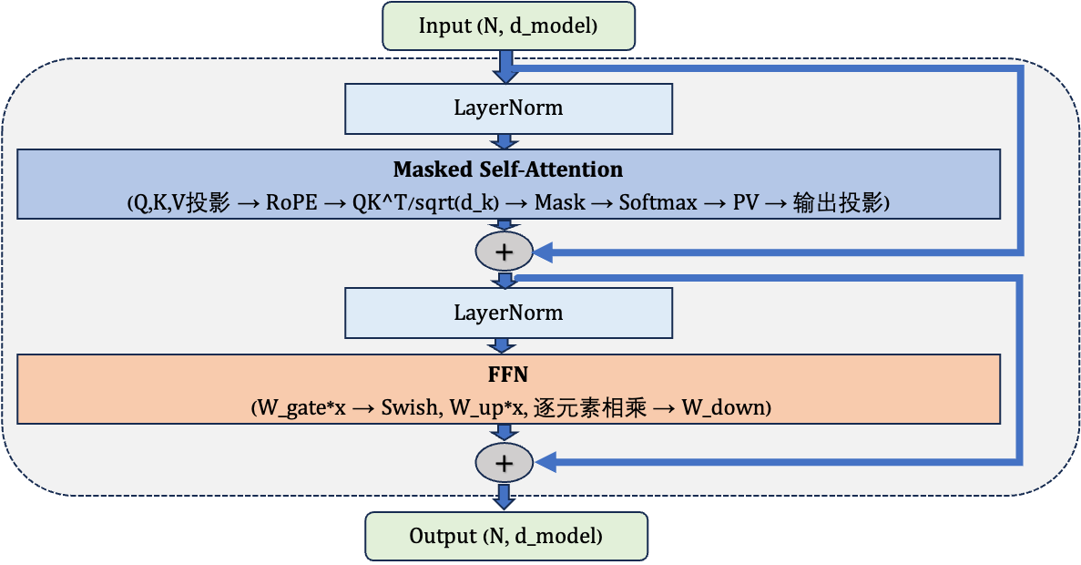
A few details worth noticing:
🍎 RMSNorm instead of LayerNorm. LLaMA and most later models use RMSNorm (Root Mean Square Normalization): skip mean subtraction, keep only divide-by-RMS. Simpler compute, similar quality.
🍎 RoPE only on Q and K. Rotary position encoding makes the Q·K product carry relative position. V does not need rotation, because V carries content, not the position-matching signal.
🍎 Pre-Norm residual paths stay clean. Both residual paths in the figure come straight from the Add node, with no transform in between. Gradients can travel back along the residual path without loss. That is key to stable deep training.
3. Causal Mask: how causal masking works
3.1 Why you need a causal mask
Decoder-only training is “given previous tokens, predict the next.” When computing Attention for token i, it may only see positions 0 through i. It must not peek at i+1 and beyond; otherwise the prediction task becomes an open-book exam and the model learns nothing.
That constraint matches natural language generation: when you say the fifth character, you genuinely do not know the sixth. The model must obey the same causal order.
At training time, for efficiency, we feed the whole sequence at once and compute in parallel (not token by token). Parallelism means every token’s Attention is computed together; without a limit, every token would see the full sequence. The Causal Mask enforces “only look at the past” while still allowing parallel compute.
3.2 Visualizing the mask matrix
Suppose sequence length is 5. The Attention score matrix S has shape (5, 5). S[i][j] is the raw attention score of token i to token j. Causal masking requires: when j > i (j is after i), S[i][j] must be masked.
The mask matrix M looks like this (0 means keep, -inf means mask):
Token:   t0    t1    t2    t3    t4
t0  [  0   -inf  -inf  -inf  -inf ]
t1  [  0     0   -inf  -inf  -inf ]
t2  [  0     0     0   -inf  -inf ]
t3  [  0     0     0     0   -inf ]
t4  [  0     0     0     0     0  ]
After adding M to S, masked positions become negative infinity. In softmax, , so those attention weights become zero.
Another view: which positions are visible (1 = visible, 0 = invisible):
Token:   t0   t1   t2   t3   t4
t0  [  1    0    0    0    0  ]    t0 can only see itself
t1  [  1    1    0    0    0  ]    t1 can see t0 and itself
t2  [  1    1    1    0    0  ]    t2 can see t0, t1, and itself
t3  [  1    1    1    1    0  ]    t3 can see everything before and itself
t4  [  1    1    1    1    1  ]    t4 can see everything
This is a lower-triangular matrix, so the causal mask is also called a “lower-triangular mask” or “upper-triangular mask” (depending on whether you mean the kept region or the masked region).
3.3 How to implement it
In code, causal masking is short:
import torch

def create_causal_mask(seq_len, device='cuda'):
    """Create a causal mask: upper triangle is -inf, the rest is 0"""
    # torch.triu takes the upper triangle; diagonal=1 starts one row above the main diagonal
    mask = torch.triu(
        torch.full((seq_len, seq_len), float('-inf'), device=device),
        diagonal=1
    )
    return mask

# Example: seq_len = 4
# tensor([[  0., -inf, -inf, -inf],
#         [  0.,   0., -inf, -inf],
#         [  0.,   0.,   0., -inf],
#         [  0.,   0.,   0.,   0.]])
At use time, add it to the Attention scores:
scores = torch.matmul(Q, K.transpose(-2, -1)) / math.sqrt(d_k)
scores = scores + create_causal_mask(seq_len, device=scores.device)
attn_weights = torch.softmax(scores, dim=-1)
In high-performance implementations (such as FlashAttention), the causal mask is not built as an explicit N×N matrix and added. During tiled compute, index checks skip the upper triangle that does not need work, which saves VRAM and cuts useless compute.
4. PyTorch implementation: build a Decoder Block from scratch
Below is a complete, runnable Transformer Decoder Block with Pre-Norm (RMSNorm), Masked Multi-Head Attention (with RoPE), SwiGLU FFN, and residual connections.
import torch
import torch.nn as nn
import torch.nn.functional as F
import math

class RMSNorm(nn.Module):
    """RMSNorm: RMS normalization only; skip mean subtraction"""

    def __init__(self, d_model: int, eps: float = 1e-6):
        super().__init__()
        self.eps = eps
        self.weight = nn.Parameter(torch.ones(d_model))

    def forward(self, x: torch.Tensor) -> torch.Tensor:
        # x: (batch, seq_len, d_model)
        rms = torch.sqrt(x.pow(2).mean(dim=-1, keepdim=True) + self.eps)
        return x / rms * self.weight

def precompute_rope_freqs(d_k: int, max_seq_len: int, theta: float = 10000.0):
    """Precompute RoPE rotation frequencies"""
    # Frequency: theta_i = 1 / (theta ^ (2i / d_k)), i = 0, 1, ..., d_k/2 - 1
    freqs = 1.0 / (theta ** (torch.arange(0, d_k, 2).float() / d_k))
    # Position indices: 0, 1, ..., max_seq_len - 1
    positions = torch.arange(max_seq_len).float()
    # Outer product: (max_seq_len, d_k // 2)
    angles = torch.outer(positions, freqs)
    # Return cos and sin, both shape (max_seq_len, d_k // 2)
    return torch.cos(angles), torch.sin(angles)

def apply_rope(x: torch.Tensor, cos: torch.Tensor, sin: torch.Tensor):
    """
    Apply rotary position encoding to Q or K
    x: (batch, seq_len, num_heads, d_k)
    cos, sin: (seq_len, d_k // 2)
    """
    seq_len = x.shape[1]
    cos = cos[:seq_len].unsqueeze(0).unsqueeze(2)  # (1, seq, 1, d_k//2)
    sin = sin[:seq_len].unsqueeze(0).unsqueeze(2)

    # Split the last dim of x into two halves
    x1 = x[..., : x.shape[-1] // 2]
    x2 = x[..., x.shape[-1] // 2 :]

    # Rotation: (x1 * cos - x2 * sin, x1 * sin + x2 * cos)
    rotated = torch.cat([x1 * cos - x2 * sin, x1 * sin + x2 * cos], dim=-1)
    return rotated

class MaskedMultiHeadAttention(nn.Module):
    """Multi-head attention with a causal mask"""

    def __init__(self, d_model: int, num_heads: int):
        super().__init__()
        assert d_model % num_heads == 0
        self.d_model = d_model
        self.num_heads = num_heads
        self.d_k = d_model // num_heads

        self.W_Q = nn.Linear(d_model, d_model, bias=False)
        self.W_K = nn.Linear(d_model, d_model, bias=False)
        self.W_V = nn.Linear(d_model, d_model, bias=False)
        self.W_O = nn.Linear(d_model, d_model, bias=False)

    def forward(self, x: torch.Tensor, rope_cos: torch.Tensor,
                rope_sin: torch.Tensor) -> torch.Tensor:
        batch, seq_len, _ = x.shape

        # Linear projections
        Q = self.W_Q(x)  # (batch, seq, d_model)
        K = self.W_K(x)
        V = self.W_V(x)

        # Split into heads: (batch, seq, num_heads, d_k)
        Q = Q.view(batch, seq_len, self.num_heads, self.d_k)
        K = K.view(batch, seq_len, self.num_heads, self.d_k)
        V = V.view(batch, seq_len, self.num_heads, self.d_k)

        # Apply RoPE (Q and K only)
        Q = apply_rope(Q, rope_cos, rope_sin)
        K = apply_rope(K, rope_cos, rope_sin)

        # Transpose to (batch, num_heads, seq, d_k) for batched matmul
        Q = Q.transpose(1, 2)
        K = K.transpose(1, 2)
        V = V.transpose(1, 2)

        # Attention scores: (batch, num_heads, seq, seq)
        scores = torch.matmul(Q, K.transpose(-2, -1)) / math.sqrt(self.d_k)

        # Causal mask
        causal_mask = torch.triu(
            torch.full((seq_len, seq_len), float('-inf'), device=x.device),
            diagonal=1
        )
        scores = scores + causal_mask.unsqueeze(0).unsqueeze(0)

        # Softmax + weighted sum
        attn_weights = F.softmax(scores, dim=-1)
        output = torch.matmul(attn_weights, V)  # (batch, heads, seq, d_k)

        # Merge heads: (batch, seq, d_model)
        output = output.transpose(1, 2).contiguous().view(batch, seq_len, -1)

        # Output projection
        return self.W_O(output)

class SwiGLUFFN(nn.Module):
    """SwiGLU feed-forward: three linear layers + gated activation"""

    def __init__(self, d_model: int, ffn_dim: int):
        super().__init__()
        self.W_gate = nn.Linear(d_model, ffn_dim, bias=False)
        self.W_up = nn.Linear(d_model, ffn_dim, bias=False)
        self.W_down = nn.Linear(ffn_dim, d_model, bias=False)

    def forward(self, x: torch.Tensor) -> torch.Tensor:
        # gate path: activate with SiLU (= Swish with beta=1)
        gate = F.silu(self.W_gate(x))    # (batch, seq, ffn_dim)
        # up path: linear transform, no activation
        up = self.W_up(x)                # (batch, seq, ffn_dim)
        # gated multiply + project down
        return self.W_down(gate * up)    # (batch, seq, d_model)

class TransformerDecoderBlock(nn.Module):
    """Full Pre-Norm Transformer Decoder Block"""

    def __init__(self, d_model: int, num_heads: int, ffn_dim: int,
                 norm_eps: float = 1e-6):
        super().__init__()
        self.norm1 = RMSNorm(d_model, eps=norm_eps)
        self.attn = MaskedMultiHeadAttention(d_model, num_heads)
        self.norm2 = RMSNorm(d_model, eps=norm_eps)
        self.ffn = SwiGLUFFN(d_model, ffn_dim)

    def forward(self, x: torch.Tensor, rope_cos: torch.Tensor,
                rope_sin: torch.Tensor) -> torch.Tensor:
        # First sublayer: RMSNorm -> Masked MHA -> residual
        h = x + self.attn(self.norm1(x), rope_cos, rope_sin)
        # Second sublayer: RMSNorm -> SwiGLU FFN -> residual
        out = h + self.ffn(self.norm2(h))
        return out

# ---------- Sanity check: instantiate with LLaMA-2-7B config ----------
if __name__ == "__main__":
    d_model = 4096
    num_heads = 32
    ffn_dim = 11008
    max_seq_len = 4096
    d_k = d_model // num_heads  # 128

    block = TransformerDecoderBlock(d_model, num_heads, ffn_dim)

    # Precompute RoPE
    rope_cos, rope_sin = precompute_rope_freqs(d_k, max_seq_len)

    # Fake input: batch=2, seq_len=128
    x = torch.randn(2, 128, d_model)
    output = block(x, rope_cos, rope_sin)

    print(f"Input shape:  {x.shape}")       # (2, 128, 4096)
    print(f"Output shape: {output.shape}")   # (2, 128, 4096)

    # Count parameters
    total_params = sum(p.numel() for p in block.parameters())
    print(f"Single block params: {total_params:,}")  # ~201M
A few key points in the code:
- RMSNorm has one learnable parameter
weight(that is ), no bias. It computes RMS over each token’s feature vector, then normalizes. - RoPE is precomputed and adds no learnable parameters. Only Q and K are rotated; V stays as is.
- SwiGLU FFN has three weight matrices. output goes through SiLU, then multiplies elementwise with output (the gate), and projects down.
- Residual connections in the Block
forwardare plain adds:h = x + self.attn(self.norm1(x), ...).
5. Dimension configs across popular models
Models of different sizes are the same Decoder Block structure with different dimensions. The table below summarizes key parameters of a few landmark models:
| Model | max_seq_len | |||||||
|---|---|---|---|---|---|---|---|---|
| LLaMA-2-7B | 4096 | 32 | 32 (MHA) | 128 | 32 | 11008 | 32000 | 4096 |
| LLaMA-2-13B | 5120 | 40 | 40 (MHA) | 128 | 40 | 13824 | 32000 | 4096 |
| LLaMA-2-70B | 8192 | 64 | 8 (GQA) | 128 | 80 | 28672 | 32000 | 4096 |
| GPT-3 175B | 12288 | 96 | 96 (MHA) | 128 | 96 | 49152 | 50257 | 2048 |
| Mistral-7B | 4096 | 32 | 8 (GQA) | 128 | 32 | 14336 | 32000 | 32768 |
Patterns worth noticing:
🍎 (per-head dim) stays at 128. No matter how large the model, each attention head works in 128 dims. Growth comes from more heads () and more layers (), not larger per-head dim. 128 dims is already enough for each head to capture a meaningful attention pattern.
🍎 Ratio of to . In the standard Transformer, . With SwiGLU, to keep total parameters similar (three matrices vs two), people usually take , then round up to a convenient number. For LLaMA-2-7B, , rounded to 11008 (a multiple of 256, better for GPU alignment). Mistral-7B uses , a bit larger by design choice.
🍎 GQA arrives. LLaMA-2-70B and Mistral-7B use Grouped-Query Attention: fewer KV heads than Q heads. LLaMA-2-70B uses 8 KV heads for 64 Q heads (8 Q heads share one KV group), cutting KV Cache to 1/8 of MHA and sharply reducing inference VRAM.
6. Hand-calculating parameter counts
Hand-counting model parameters is basic skill for an AI Infra engineer. Parameter count lets you estimate VRAM, communication cost, and training cost.
6.1 Deriving the general formulas
A standard Decoder-only model has these parts:
(1) ❇️ Token Embedding layer
Maps token IDs to vectors:
where is vocab size and is .
(2) ❇️ One Decoder Block
For a Block with MHA (independent KV per head) and SwiGLU FFN:
Attention: four projection matrices (no bias):
Why ? , , , are each , so each has parameters.
With GQA (KV heads , Q heads , head dim ):
SwiGLU FFN: three matrices (no bias):
where is the FFN intermediate dim.
RMSNorm (two of them, params each):
Per Block total:
(3) ❇️ Final RMSNorm + output head (LM Head)
First term is final RMSNorm; second is the LM Head (maps to ).
(4) ❇️ Total model parameters
where is layer count. If Embedding and LM Head share weights (Weight Tying), subtract one .
6.2 Worked example: LLaMA-2-7B
Config reminder: , , , , ,
🍓 Attention params (one Block):
| Matrix | Shape | Params |
|---|---|---|
| 4096 x 4096 | 16,777,216 | |
| 4096 x 4096 | 16,777,216 | |
| 4096 x 4096 | 16,777,216 | |
| 4096 x 4096 | 16,777,216 | |
| Attention subtotal | 67,108,864 (67.1M) |
Check:
🍓 FFN params (one Block):
| Matrix | Shape | Params |
|---|---|---|
| 4096 x 11008 | 45,088,768 | |
| 4096 x 11008 | 45,088,768 | |
| 11008 x 4096 | 45,088,768 | |
| FFN subtotal | 135,266,304 (135.3M) |
Check:
🍓 RMSNorm params (one Block):
🍓 One Block total:
= 202,383,360 (~202M)
FFN share = 135.3M / 202.4M = 66.8%, Attention share = 67.1M / 202.4M = 33.2%
🍓 Full model:
| Component | Calculation | Params |
|---|---|---|
| Token Embedding | 131,072,000 | |
| 32 Blocks | 6,476,267,520 | |
| Final RMSNorm | 4096 | 4,096 |
| LM Head | 131,072,000 | |
| Total | 6,738,415,616 (~6.74B) |
LLaMA-2 keeps Embedding and LM Head as two separate weight sets (no tying), so 6.74B already includes two copies of 131M, matching the published count. With weight tying you would subtract 131M, about 6.61B. The official “7B” label is an approximation.
6.3 Exercise: LLaMA-2-13B parameter count
Config: , , , , ,
Try it yourself first, then check the answer below:
One Block:
- Attention: (104.9M)
- FFN: (212.3M)
- RMSNorm:
- One Block total: (~317M)
Full model:
- Embedding:
- 40 Blocks:
- Final RMSNorm:
- LM Head:
- Total: (~13.0B)
Matches the official 13B label.
6.4 Weight Tying
Many models share one weight matrix between Token Embedding and LM Head. That trick is Weight Tying, proposed by Press and Wolf in 2017.
Intuition: Embedding maps token IDs to semantic vectors (discrete → continuous). LM Head maps semantic vectors back to token probabilities (continuous → discrete). The two ops are inverses, so sharing the same matrix (forward vs transpose) is reasonable.
Benefits of Weight Tying:
- Fewer parameters: for , , you save 131M params, about 2% of a 7B model
- Regularization: shared weights are an implicit constraint that keeps Embedding space and output space from drifting apart
- Less VRAM: one fewer matrix to store
GPT-2 uses Weight Tying; LLaMA-2 does not (tie_word_embeddings: false in HuggingFace configs). Whether to use it depends on vocab size relative to model size. When the vocab is small vs the model (32000 vs 7B), the parameter savings are small, but the regularization effect can still matter.
7. Estimating FLOPs
Parameter count tells you VRAM. FLOPs tell you training time and hardware utilization.
7.1 FLOPs of a matmul
The base of FLOPs estimates is matrix multiply. For :
- The result has elements
- Each element needs multiplies and adds
- Total FLOPs ≈ (count multiply and add as one FLOP each)
7.2 FLOPs of one forward pass
For a Transformer with parameters processing a sequence of length , forward FLOPs are roughly:
That is the "" rule of thumb. Intuition: most compute is matmul; each parameter takes part in one matmul in the forward pass and contributes about 2 FLOPs (one mul, one add), then multiply by tokens.
More precisely, only counts linear-layer (GEMM) FLOPs and ignores Attention and (those scale with sequence length squared). The fuller formula is:
The second term is Attention (per layer per head: two matmuls, each , total ). When is short (say 2048), the second term is much smaller than the first, so "" is a good approximation. When is long (e.g. 128K), Attention compute can approach or exceed the linear layers.
7.3 Training vs inference FLOPs
✳️ Training FLOPs
Training is forward plus backward. Empirically, backward is about 2× forward (gradients w.r.t. weights and inputs). So:
For a full run over tokens:
Example: LLaMA-2-7B trained on 2 trillion tokens:
- FLOPs
On 1000 A100s (BF16 peak 312 TFLOPS each, assume MFU=50%):
- Effective FLOPS FLOPS
- Training time seconds ≈ 6 days
That matches the order of magnitude of publicly reported training times.
✳️ Inference FLOPs
Inference is forward only, about FLOPs per token. The catch in Decode: each step processes 1 token, so matmul becomes matrix-vector multiply (GEMV). The GPU is far from compute-saturated; the bottleneck is memory bandwidth, not peak FLOPS. Inference optimization therefore focuses on memory bandwidth (Memory Bound), not peak compute.
7.4 Worked estimate
LLaMA-2-7B inference on A100-80GB:
- Single-token Decode FLOPs GFLOPs
- A100 FP16 peak TFLOPS
- In theory FLOPs only need
In practice one token Decode takes about 10-20ms. Why hundreds of times off? Decode is Memory Bound: you must move all model weights from HBM (13.4 GB FP16). A100 HBM bandwidth is 2 TB/s, so weight movement alone is 13.4 GB / 2 TB/s = 6.7ms. Add KV Cache traffic and other overhead, and 10-20ms is reasonable.
8. VRAM planning in detail
VRAM planning is one of the most common AI Infra ops questions: given a model and one (or more) GPUs, does it fit, and if not, what do you do?
8.1 Model weight VRAM
Weight VRAM depends on parameter count and storage precision:
| Precision | Bytes per param | 7B weights | 13B weights | 70B weights |
|---|---|---|---|---|
| FP32 | 4 Bytes | 26.8 GB | 52.0 GB | 280.0 GB |
| FP16 / BF16 | 2 Bytes | 13.4 GB | 26.0 GB | 140.0 GB |
| INT8 | 1 Byte | 6.7 GB | 13.0 GB | 70.0 GB |
| INT4 | 0.5 Bytes | 3.35 GB | 6.5 GB | 35.0 GB |
Formula: VRAM = param_count × bytes_per_param
FP16 and BF16 are both 16-bit floats and use the same VRAM. BF16 has more exponent bits (8 vs FP16’s 5), so a wider range and less overflow risk in training; it is the mainstream training choice today.
8.2 Training VRAM: four main pieces
Training needs far more VRAM than weights alone. For mixed-precision training (BF16 weights + FP32 optimizer):
(1) Model weights: 2 Bytes/param
Weights stored in BF16: Bytes ( = param count).
(2) Gradients: 2 Bytes/param
Same shape as weights, BF16: Bytes.
(3) Optimizer state: depends on the optimizer
This is the big consumer. For Adam/AdamW, you keep three things:
- FP32 parameter copy (Master Weights): Bytes. Why FP32? BF16 has only about 3-4 significant digits. If lr × grad is tiny (say 1e-5), BF16 cannot represent the update and it rounds away. FP32 has about 7 significant digits and can capture those small updates.
- First moment (m): Bytes. Adam’s EMA of gradients, estimating the mean.
- Second moment (v): Bytes. Adam’s EMA of squared gradients, estimating variance for adaptive learning rates.
Optimizer state total: = Bytes.
When people say “Adam needs 4× parameter VRAM,” they mean roughly ≈ 3-4× extra relative to weights+grads; the optimizer state alone is 6× the BF16 weights .
(4) Activation Memory
Forward activations must be kept for backward. Activation VRAM scales with batch_size and sequence length. A rough formula:
where is sequence length, is batch_size, is , is layers, and is a constant (about 10-14, depending on Activation Checkpointing).
For LLaMA-2-7B, seq_len=2048, batch_size=4, no Activation Checkpointing:
- Rough Bytes (BF16)
- GB
With Activation Checkpointing (keep only per-layer inputs, recompute intermediates on backward), activation VRAM can drop to about 1/3 to 1/5, at the cost of ~33% more compute.
✳️ Training VRAM summary (LLaMA-2-7B, 6.7B params):
| Component | How computed | VRAM |
|---|---|---|
| BF16 model weights | 13.4 GB | |
| BF16 gradients | 13.4 GB | |
| FP32 Master Weights | 26.8 GB | |
| Adam first moment (FP32) | 26.8 GB | |
| Adam second moment (FP32) | 26.8 GB | |
| Static total | 107.2 GB | |
| Activation (estimate) | batch=4, seq=2048 | ~25.8 GB |
| Grand total | ~133 GB |
133 GB already exceeds one A100-80GB. That is why training a “small” 7B model still needs distributed training (ZeRO, tensor parallelism, etc.).
8.3 Inference VRAM: weights + KV Cache
Inference needs neither gradients nor optimizer state, so VRAM is much simpler:
(1) Model weights
FP16 example: 6.7B × 2 = 13.4 GB
(2) KV Cache
Each token caches one K and one V vector per layer:
For LLaMA-2-7B (MHA, ):
- Per token: Bytes = 512 KB
- seq_len = 4096: KB = 2 GB
- batch_size = 16: GB = 32 GB
✳️ Inference VRAM summary:
| Component | LLaMA-2-7B (FP16) | LLaMA-2-7B (INT4) |
|---|---|---|
| Model weights | 13.4 GB | 3.35 GB |
| KV Cache (seq=4096, batch=16) | 32 GB | 32 GB (KV usually still FP16) |
| Other overhead (framework, buffers) | ~1 GB | ~1 GB |
| Total | ~46.4 GB | ~36.4 GB |
Note: even if weights are INT4, KV Cache usually stays FP16, because quantizing KV hurts quality more. Recent work (KIVI, KVQuant) compresses KV Cache to INT4 or even INT2, but needs extra calibration and quality checks.
8.4 Full planning case
Scenario: deploy LLaMA-2-13B for inference on one A100-80GB, target batch_size=8, max sequence length 4096. Does it fit?
Step 1, model weights:
- 13B params × 2 Bytes (FP16) = 26 GB
Step 2, KV Cache:
- LLaMA-2-13B: , (MHA),
- Per-token KV: Bytes = 800 KB
- seq=4096, batch=8: GB
Step 3, framework overhead:
- CUDA context + framework buffers + temps ≈ 2 GB
Step 4, sum:
- 26 + 25.6 + 2 = 53.6 GB
✳️ Conclusion: 53.6 GB < 80 GB, it fits, with about 26 GB headroom.
What if you raise batch_size to 16?
- KV Cache doubles: GB
- Total: GB
Very close to the 80 GB limit, almost no headroom; OOM is likely in practice. Options then:
- INT8 quantize weights: GB, total 66.2 GB, workable
- Use a GQA model (e.g. Mistral) to shrink KV Cache
- Quantize KV Cache
- Lower max sequence length
That is the real value of VRAM planning: not guessing “it should run,” but computing each cost, finding the bottleneck, and picking a fitting optimization.
9. Architecture comparison of popular open-source models
Finally, one table of current mainstream open-source LLM architecture choices for a global view:
| Feature | LLaMA-2 | LLaMA-3 | Mistral-7B | Qwen-2.5 | DeepSeek-V3 |
|---|---|---|---|---|---|
| Attention type | MHA (7B/13B) / GQA (70B) | GQA | GQA | GQA | MLA (Multi-head Latent Attention) |
| KV heads (7B-class) | 32 (MHA) | 8 | 8 | 4 | — (MLA compresses KV) |
| Position encoding | RoPE | RoPE | RoPE | RoPE | RoPE |
| Normalization | RMSNorm (Pre-Norm) | RMSNorm (Pre-Norm) | RMSNorm (Pre-Norm) | RMSNorm (Pre-Norm) | RMSNorm (Pre-Norm) |
| FFN type | SwiGLU | SwiGLU | SwiGLU | SwiGLU | SwiGLU + MoE |
| MoE? | No | No | Mixtral variant yes | Some variants yes | Yes (256 experts, Top-8) |
| Vocab size | 32000 | 128256 | 32000 | 151936 | 129280 |
| Max context | 4096 | 8192 (extendable) | 32768 (Sliding Window) | 32768+ | 128K+ |
| Special design | — | Larger vocab, longer context | Sliding Window Attention | Expand on demand | MLA + MoE combo |
Key trends:
GQA becomes default. From LLaMA-2 MHA to almost all later models using GQA, the driver is inference KV Cache VRAM. KV heads fell from 32 to 8 or even 4, cutting KV Cache 4-8×.
Vocab keeps growing. LLaMA-2’s 32000 to LLaMA-3’s 128256: larger vocab means better multilingual coverage and higher token efficiency (same text in fewer tokens), but also a larger Embedding layer.
MoE rises. DeepSeek-V3 and Mixtral use mixture-of-experts: more total params, fewer activated params per token (only a few experts fire), for better quality. That brings new distributed training and inference challenges (Expert Parallelism, load balancing, etc.).
MLA innovation. DeepSeek-V3’s Multi-head Latent Attention projects KV into a low-dim latent space and recovers it, cutting KV Cache a lot while keeping capability. It is a further step along the GQA idea.
🎯 Self-check list
After this article, check that you can:
- Explain why Decoder-only won in the large-model era, with at least three reasons
- Draw a full Decoder Block data-flow diagram on a whiteboard, labeling RMSNorm, Masked MHA, SwiGLU FFN, and residual order
- Draw a causal mask matrix (for sequence length ) and explain what upper-triangle does
- Hand-calculate LLaMA-2-7B and 13B parameter counts (within 5%), and state the FFN vs Attention parameter ratio
- Estimate training FLOPs with "" and inference FLOPs with ""
- Compute weight VRAM for a given model in FP16, INT8, and INT4
- Compute how much VRAM Adam needs, and explain why FP32 Master Weights are required
- Given a model config and GPU SKU, finish a full VRAM plan (weights + KV Cache, or weights + grads + optimizer + Activation) and decide whether it fits
📚 References
Papers
- Attention Is All You Need (Vaswani et al., 2017): https://arxiv.org/abs/1706.03762 — Original Transformer paper
- LLaMA 2: Open Foundation and Fine-Tuned Chat Models (Touvron et al., 2023): https://arxiv.org/abs/2307.09288 — LLaMA-2 technical report
- Mistral 7B (Jiang et al., 2023): https://arxiv.org/abs/2310.06825 — Mistral architecture and Sliding Window Attention
- GLU Variants Improve Transformer (Shazeer, 2020): https://arxiv.org/abs/2002.05202 — SwiGLU activation
- Using the Output Embedding to Improve Language Models (Press & Wolf, 2017): https://arxiv.org/abs/1608.05859 — Weight Tying
- Scaling Laws for Neural Language Models (Kaplan et al., 2020): https://arxiv.org/abs/2001.08361 — Scaling of model size and performance
- ZeRO: Memory Optimizations Toward Training Trillion Parameter Models (Rajbhandari et al., 2020): https://arxiv.org/abs/1910.02054 — ZeRO memory optimization
- DeepSeek-V3 Technical Report (DeepSeek-AI, 2024): https://arxiv.org/abs/2412.19437 — MLA + MoE architecture
Tutorials and blogs
- The Illustrated Transformer (Jay Alammar): https://jalammar.github.io/illustrated-transformer/
- Transformer Math 101 (EleutherAI): https://blog.eleuther.ai/transformer-math/ — Detailed parameter and FLOPs derivations
- LLM Training: FSDP vs DeepSpeed (Hugging Face): https://huggingface.co/docs/transformers/main/en/perf_train_gpu_many