6.1 Inference parallelism overview
From a memory ledger and latency/throughput goals, compare how TP, PP, DP, and EP store data, communicate, and fit different cases; give an order for picking parallel degrees and a runnable estimation script
The first five chapters assumed one thing: the model fits on a single GPU. At Dense 70B scale, or MoE models like DeepSeek-V3, that assumption fails, and the engine has to split the model across cards—or even machines.
There is more than one way to split. Slice inside a layer, slice between layers, replicate whole copies, or slice by expert: each fixes a different problem, and the communication cost differs a lot. This section first makes clear why you split, then puts the four approaches side by side, and finally gives an order for choosing parallel degrees. Sections 6.2–6.4 unpack each one.
⏰ Currency: The principles do not depend on any framework; vLLM advice and parameters follow the v0.32.0 docs (released 2026-10-18).
📑 Contents
- 1. Two starting points: does not fit, or not fast enough
- 2. Inference parallelism and training parallelism have different goals
- 3. Four splits side by side
- 4. Communication ledger: how much each step moves
- 5. Order for choosing parallel degrees
- 6. Hands-on estimate: does one card fit
- Summary
- Self-check list
- References
1. Two starting points: does not fit, or not fast enough
1.1 Does not fit: count weights and KV Cache together
Take Llama-3.1-70B. It has 80 layers, hidden size 8192, 64 Q heads and 8 KV heads (GQA), 128 dims per head. In BF16 the weights alone are about 70.6B × 2 B ≈ 141 GB—too much for a single 80 GB H100.
The KV Cache ledger was worked out in Chapter 1. Each token stores one K and one V per layer:
A 32K-token request needs 10 GiB; eight such requests concurrent need 80 GiB. Once weights fit, leftover memory decides how many requests you can serve at once.
So “fits” has at least two layers of meaning:
- Weights fit: each card’s share of weights is under GPU memory—that is the prerequisite to start at all.
- KV Cache is enough: after weights, activations, CUDA Graph, and other overhead, what remains must cover the target concurrency and context length. Often the GPU count is pushed up by this second constraint.
1.2 Not fast enough: single-card bandwidth caps Decode
Chapter 1’s Roofline analysis said small-batch Decode is memory-bound: every generation step must read the full weights from HBM once. H100 SXM HBM3 bandwidth is about 3.35 TB/s; if a 70B model somehow fit on one card, reading 141 GB once would still take 42 ms, so TPOT cannot go below that.
Slice the weights across 4 cards and each card reads about 35 GB per step; four cards read in parallel, so in theory the memory time per step drops to about ¼. That is where “faster after splitting” comes from; the cost is syncing across cards.
Another kind of “not fast enough” is throughput: one replica’s latency is fine, but there are too many requests. Then you do not need to slice the model—just run more replicas.
📌 Key point: First tell which problem you have. Weights do not fit or KV is short → slice the model. Single-request latency is too high → let several cards compute one request together. Aggregate throughput is short → add replicas. The three problems map to different parallelism.
2. Inference parallelism and training parallelism have different goals
Module 3 covered TP, PP, DP, and EP. The names and the slicing patterns are basically the same for inference. What differs is what each side optimizes:
| 📊 Dimension | Training | Inference |
|---|---|---|
| What sits in memory | Weights + gradients + optimizer state + activations | Weights + KV Cache; almost no gradients or optimizer state |
| Main goal | Samples per unit time, and eventual convergence | Latency percentiles for TTFT and TPOT, plus throughput under SLOs |
| Work per step | Forward + backward on a large batch | Decode has only 1 new token per request; work is small and load-dependent |
| What DP syncs | AllReduce gradients every step | Replicas do not sync (Dense models) |
| PP bubble | Amortized with many micro-batches | Decode step depends on step ‘s sample; you need several batches interleaved to fill the pipe |
| ZeRO / FSDP | Common: trade communication for memory | Rarely used: every step would re-gather weights, and Decode cannot afford that traffic |
On the last row: FSDP shards weights and temporarily AllGathers full parameters before compute. Training has enough compute per step to hide that gather; Decode computes only tens of tokens per step but would move the full weights over the network, so communication dwarfs compute. Inference therefore shards weights with TP and PP, not ZeRO-style sharding.
💡 Tip: Training cares about “samples per second on average”; inference cares about “how long each user waits.” For the same parallelism, judge it by effect on TTFT and TPOT, and by how much concurrency you can serve under latency constraints.
3. Four splits side by side
A kitchen analogy first. One table of dishes is cooked by a crew:
- TP: Several people share one step—each chops part of the vegetables, then they must gather before anything goes in the pan. Fast, but every step needs a meetup.
- PP: Stages in a line—one preps, one stir-fries, one plates. Each owns a segment and hands off once, but with only one table the earlier cooks sit idle; you need several tables in flight to keep everyone busy.
- DP: Open several identical shops; each takes its own guests, no interference.
- EP: Stations by cuisine—Sichuan cooks only cook Sichuan. Every dish goes to the right station and comes back when done.
On the model, the figure below draws the four splits on 4 GPUs and an 80-layer model; color is which GPU owns that cell:
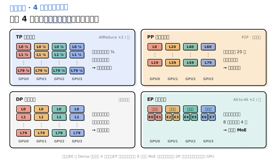
| 📊 Method | What it slices | Weights per card | Communication in forward | Main win |
|---|---|---|---|---|
| TP | Weight matrices per layer, by heads or intermediate dim | About | 2 AllReduces per layer | Less weight read per card; single-request latency drops |
| PP | Layers, contiguous stages | About | Point-to-point activations between stages | Little communication; good for cross-node scale-out |
| DP | Nothing; full replicas | One full copy | None for Dense models | Throughput grows with replica count |
| EP | Experts in MoE layers | Experts about ; attention and shared parts counted separately | 2 All-to-Alls per MoE layer | Fits MoE models with a huge expert pool |
A few notes:
- TP and PP both cut per-card weight memory, but only TP lets several cards process the same token at once, so only TP directly lowers single-request TPOT. Under PP a token walks the stages in order; single-request latency does not get shorter.
- DP does not save memory. It assumes one replica already fits, and can combine with TP/PP—for example two replicas at TP=4 each.
- EP only applies to MoE layers. Attention still needs TP or DP; a common vLLM pattern is attention on DP and experts on EP (section 6.4).
4. Communication ledger: how much each step moves
Let this step’s batch have tokens (for Decode, that is concurrent requests), hidden size , and bytes per activation element.
4.1 TP: many calls, each small
Each layer does 2 AllReduces; each reduces a tensor of size:
An -layer model does per step. With a Ring algorithm each card sends about bytes per call. For Llama-3.1-70B, TP=4, and 64 Decode requests:
- Each AllReduce:
- 160 calls per step; each card sends about
At H100 NVLink unidirectional 450 GB/s, pure transfer is about 0.56 ms—small next to a TPOT of tens of ms. But 160 calls each need every card to align, messages are tiny, and fixed launch/sync latency dominates. That is why TP inside a node leans on NVLink and is hard to use well across nodes (section 6.2).
4.2 PP: few calls, only at stage boundaries
Each stage boundary sends activations once: point-to-point sends per step. vLLM’s Llama path passes hidden_states and residual between stages—about 2 MiB per boundary at 64 requests. Call count drops from 160 to 3, so network demands are much lower.
PP’s cost is not volume but the bubble: while a batch is in stage 2, stage 1 waits. Section 6.3 covers filling the pipe by interleaving multiple batches.
4.3 EP: large volume, and uneven
Each MoE layer does Dispatch then Combine. Every token goes to the expert cards it chose, bytes each, then comes back on Combine:
For DeepSeek-V3 (, 8 routed experts active per token), BF16 round-trip per token per MoE layer is about 229 KB; the portion that stays on the local card never hits the network. Versus TP, EP call counts are similar (2 per MoE layer; none on Dense layers), but each message is larger and route-dependent: hot-expert cards receive more, and the layer waits on the busiest card (section 6.4).
4.4 DP: zero communication on Dense models
Each replica handles its own requests; no sync in the forward pass. MoE with DP + EP is different: every DP rank must enter MoE layers together for All-to-All, so a rank with no work still runs an empty forward to stay in sync.
| 📊 Method | Calls per step | Size each (64 Decode tokens) | Interconnect need |
|---|---|---|---|
| TP=4 | 160 AllReduces | 1 MiB | Low latency, high bandwidth; basically inside an NVLink domain |
| PP=4 | 3 P2P | About 2 MiB | Ordinary RDMA is enough |
| DP | 0 | — | None |
| EP | 2 All-to-Alls per MoE layer | Depends on and routing | Cross-node needs RDMA and specialized communication kernels |
5. Order for choosing parallel degrees
vLLM docs for a single replica boil down to three tiers:
- Fits on one card: no distributed setup.
- Fits on one multi-GPU node: use TP; set TP to the GPU count you need.
- Does not fit on one node: TP = GPUs per node, PP = node count—TP inside the node, PP across nodes.
There is one documented exception: the model fits on one node, but GPU count does not divide the model structure (for example head count). Then you can use PP instead of TP, because PP slices by layer and allows uneven layer counts per stage.
On top of those tiers, adjust by goal:
| 🎯 Situation | Action | Why |
|---|---|---|
| One replica already meets latency; throughput is short | Add DP replicas | No inter-replica communication; scale is nearly linear |
| TPOT misses target | Raise TP (inside the NVLink domain) | Less weight read per card |
| Throughput first, latency SLO loose | Smaller TP, more replicas | TP sync cost grows with GPU count; same GPU budget often yields more total throughput as several small replicas |
| KV Cache short; concurrency stalls | Add GPUs or use PP; for GQA, once TP exceeds KV heads, KV no longer shrinks | See section 6.2 |
| MoE model | Attention DP + expert EP | Section 6.4 |
| Cross-node | Keep TP inside the node; between nodes use PP or DP/EP | TP has too many communication rounds |
⚠️ Note: Parallel degrees are also constrained by model structure. TP must divide attention head count; vLLM allows TP above KV head count at the cost of replicating KV heads. PP is not limited by heads, but when stages have uneven layer counts the slowest stage sets the pipeline rate.
6. Hands-on estimate: does one card fit
The script below follows Llama-3.1-70B’s structure and estimates per-card weights, KV size per token, and how many tokens fit in leftover space under different TP × PP mixes. Stdlib only; you can run it as-is:
GiB = 1024**3

# Llama-3.1-70B (from config.json)
MODEL = dict(params=70.6e9, layers=80, kv_heads=8, head_dim=128)
GPU_MEM = 80 * 1e9        # H100 80GB, counted as 10^9
UTIL = 0.90               # matches vLLM --gpu-memory-utilization
RESERVED = 4 * GiB        # activations, CUDA Graph, comm buffers, etc. (assumed)
DTYPE_BYTES = 2           # BF16 weights and KV


def per_gpu(tp, pp, m=MODEL):
    weights = m["params"] * DTYPE_BYTES / (tp * pp)
    kv_heads_local = max(1, m["kv_heads"] // tp)   # at least 1 head per card when TP > KV heads
    kv_per_token = 2 * (m["layers"] / pp) * kv_heads_local * m["head_dim"] * DTYPE_BYTES
    free = GPU_MEM * UTIL - weights - RESERVED
    return weights, kv_per_token, free


print(f"{'TP×PP':>6} {'wt/GPU':>9} {'KV/tok/GPU':>12} {'KV free/GPU':>11} {'tokens fit':>12} {'32K reqs':>10}")
for tp, pp in [(1, 1), (2, 1), (4, 1), (8, 1), (16, 1), (8, 2), (4, 2)]:
    w, kv, free = per_gpu(tp, pp)
    if free <= 0:
        print(f"{tp:>3}×{pp:<2} {w / GiB:>8.1f}G {'—':>12} {'no fit':>11}")
        continue
    tokens = int(free // kv)
    print(f"{tp:>3}×{pp:<2} {w / GiB:>8.1f}G {kv / 1024:>10.0f}Ki {free / GiB:>10.1f}G "
          f"{tokens:>12,} {tokens // 32768:>10}")
Output:
 TP×PP      wt/GPU   KV/tok/GPU     KV free/GPU    tokens fit    32K reqs
  1×1     131.5G            —         no fit
  2×1      65.8G            —         no fit
  4×1      32.9G         80Ki       30.2G      395,569         12
  8×1      16.4G         40Ki       46.6G    1,222,046         37
 16×1       8.2G         40Ki       54.8G    1,437,500         43
  8×2       8.2G         20Ki       54.8G    2,875,001         87
  4×2      16.4G         40Ki       46.6G    1,222,046         37
From the table:
- TP=2 still does not fit: each of two cards gets about 66 GiB of weights; with reserved space you are over. You need at least 4 cards.
- TP=4 → TP=8 roughly triples concurrency: GPU count doubles, per-card weights and KV each halve, and the two effects stack. Many deployments pick TP=8 for this reason, not only for latency.
- TP=16 only gains about 18% more tokens than TP=8: there are only 8 KV heads, so at TP=16 each card still holds 1 head; KV stops shrinking and the only extra room is from smaller weights. On the same 16 GPUs, TP=8 × PP=2 fits 2× the tokens.
- 4×2 and 8×1 have the same capacity: both use 8 GPUs and ⅛ of weights and KV per card. The difference is latency: TP=8 computes each token on 8 cards at once; 4×2 walks two TP=4 stages in sequence.
This is only a capacity estimate: weights are spread evenly by parameter count, Embedding / LM Head imbalance on PP edge stages is ignored, and the 4 GiB reserve is assumed. Real KV space is whatever vLLM prints as KV Cache capacity in the startup log.
📝 Summary
- Two motives for slicing the model: weights or KV Cache do not fit, and single-card bandwidth limits Decode. When throughput is short, add replicas; you do not have to slice the model.
- Inference does not use ZeRO/FSDP-style weight sharding: Decode compute per step is small, so temporary weight gathers cannot be hidden.
- TP does 2 AllReduces per layer and can cut single-request latency, but needs NVLink; PP only passes activations between stages, suits cross-node scale-out, and pays with bubbles; DP has zero communication on Dense models; EP does two All-to-Alls per MoE layer with volume shaped by routing.
- vLLM baseline: no split on one card; TP on one node; multi-node uses TP = GPUs per node and PP = node count.
- Once TP on a GQA model exceeds KV head count, per-card KV stops shrinking and concurrency gains from more GPUs shrink sharply.
🎯 Self-check list
- Can compute a model’s BF16 weight size and KV Cache size per token
- Can tell apart “does not fit,” “single request too slow,” and “throughput short,” and map them to slicing the model, TP, and DP
- Can explain why inference rarely uses FSDP/ZeRO weight sharding
- Can write TP’s AllReduce count per step and the size of each call
- Can explain why PP does not lower single-request TPOT
- Can pick TP and PP for single-node and multi-node deploys using vLLM’s three tiers
- Can use this section’s script to estimate KV capacity under different TP × PP and explain what changes after TP exceeds KV head count
📚 References
- Megatron-LM: Training Multi-Billion Parameter Language Models Using Model Parallelism
- GPipe: Efficient Training of Giant Neural Networks using Pipeline Parallelism
- GShard: Scaling Giant Models with Conditional Computation and Automatic Sharding
- Efficiently Scaling Transformer Inference
- The Llama 3 Herd of Models
- NVIDIA H100 Tensor Core GPU
- vLLM docs: Parallelism and Scaling