6.3 Pipeline-parallel inference
What PP stages pass between them and how much traffic that is in inference, why Decode's step dependency needs several batches in flight, uneven layer splits, single-request latency vs KV capacity, and how to choose TP×PP
TP has every card compute part of every layer. PP flips the cut: each card owns a few full layers and hands the result to the next card when done. Stages exchange activations once, so communication happens one or two orders of magnitude less often than TP. That is why PP is the main way to scale across nodes.
The cost is the pipeline itself. With one batch, only one stage works at a time and the others wait. Training fills the pipe by cutting micro-batches; Decode in inference depends on the previous step’s sample, so the fill strategy is different. This section clears that up, then covers how to split layers, how latency and capacity add up, and how to combine TP with PP.
⏰ Currency: The principles do not depend on any framework; vLLM descriptions follow v0.32.0 (released 2026-10-18).
📑 Contents
- 1. Cut by layer: what stages pass
- 2. One batch cannot fill the pipeline
- 3. How inference fills: interleave several batches
- 4. Prefill and Chunked Prefill
- 5. How to split layers: the slowest stage sets the pace
- 6. Latency, capacity, and TP×PP combinations
- 7. Hands-on: PP vs TP at the same GPU count
- Summary
- Self-check list
- References
1. Cut by layer: what stages pass
1.1 Each stage is a run of consecutive layers
PP splits layers in order into stages. Each stage sits on one card or one TP group. The first stage also owns Embedding; the last owns the final Norm, LM Head, and sampling.
A batch’s forward walks the stages in order: Stage 0 finishes its layers, sends the output to Stage 1, Stage 1 continues, until the last stage produces logits.
1.2 Only this step’s activations move
What crosses stages is the current step’s hidden state, shape , where is the token count this step. In vLLM’s Llama path, non-final stages pack the output as IntermediateTensors with two tensors, hidden_states and residual (needed for the residual connection).
KV Cache does not move. Each stage stores KV only for the layers it owns; Attention finishes inside the stage.
For Llama-3.1-70B with 64 Decode requests, each stage boundary moves per step:
At PP=2 there is only one such transfer per step, versus TP’s 160 AllReduces, so the network bar is much lower. Even on 50 GB/s InfiniBand the transfer is about 40 µs.
📌 Key point: PP communication is point-to-point one-way send; every card does not need to sync. The next stage only waits on the previous one, independent of the others.
2. One batch cannot fill the pipeline
Reuse the kitchen pipeline from section 6.1: prep, cook, plate, one person each. With one table of guests, the cook waits for prep, the plater waits for the cook. Each person works only one third of the time.
Decode in inference is worse: step ‘s input is the token sampled at step . One batch must walk all stages and sample a new token before the next step can start. With one batch, only one stage works at any moment; per-stage utilization is .
Training has bubbles too; the fix is to cut a large batch into micro-batches and feed them one after another. Inference can borrow that idea, with one limit: two adjacent steps of the same request are strictly ordered, so batches in flight must be made of different requests. Step of the same request cannot start before step has finished the pipe, no matter how you cut.
3. How inference fills: interleave several batches
3.1 Keep batches in flight
Split the running requests into groups, form independent batches, and feed them in turn. While Batch A is on Stage 1, Batch B enters Stage 0; when A reaches Stage 2, B is on Stage 1 and C enters Stage 0… Once full, every stage is busy on some batch at every moment.
The figure compares PP=4 with one batch versus four interleaved batches. Four colors are Batches A–D; the number in each cell is which Decode step that batch is on:
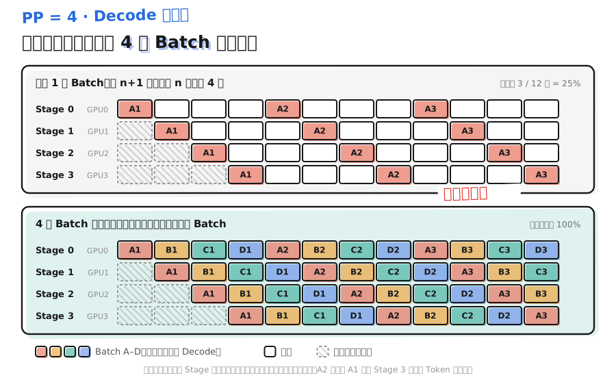
The key is the diagonal in the lower half: when A1 finishes Stage 3 and samples a token, Stage 0 is free just in time for A2. As long as in-flight batches equal stage count and stages take the same time, that rhythm holds.
3.2 What vLLM does
vLLM V1’s EngineCore turns on a batch queue when PP>1; queue length comes from max_concurrent_batches. The comment on VllmConfig.max_concurrent_batches is blunt: “PP requires PP-size concurrent batches to fill the pipeline”. The default is ; with async scheduling and the V2 Model Runner it is , the extra one overlapping schedule and execute.
The scheduler emits a new batch into Stage 0 each time; it does not wait for the previous batch’s result. A request already in an in-flight batch must finish that full pipeline pass and sample a token before its next step—exactly the step dependency from section 2.
From that: PP only helps if concurrent requests can form at least groups.
- With 1 request, no matter how large PP is, the pipeline always has one batch; utilization is .
- At concurrency 64 and PP=4, each batch has about 16 requests. Versus 64 requests computed together without PP, each forward’s batch is smaller, but all 4 stages work at once.
3.3 Uneven work creates new bubbles
The figure assumes every cell takes the same time. In practice several cases break that:
- Different work across batches: one batch has long-context requests, Attention is slower, later batches wait.
- Prefill mixed with Decode: a batch stuffed with thousands of Prefill tokens makes that cell much longer than the others.
- Requests finish or arrive: group sizes keep changing.
Any longer cell queues every later batch at that stage; the idle time is bubble. Throughput under PP is more sensitive to how balanced scheduling is.
4. Prefill and Chunked Prefill
Prefill processes a whole prompt at once and has no step dependency. As long as several requests are queued, they can interleave into the pipeline.
One very long prompt can be cut into chunks. Chunk 2 on Stage 0 only needs the KV Chunk 1 wrote on Stage 0, and that KV is already written when Chunk 1 leaves Stage 0. In principle, chunks of the same request can walk the stages one after another like a pipeline and cut TTFT on long prompts. Whether the engine schedules that way depends on the implementation; trust the version you run.
As in Chapter 2 section 2.4, Chunked Prefill block size also affects Decode stability: larger blocks make Prefill cells longer, and the unevenness in 3.3 above shows up more.
5. How to split layers: the slowest stage sets the pace
Pipeline speed is set by the slowest stage. Layer splits have a few easy-to-miss details:
- Layer count may not divide evenly: Llama-3.1-405B has 126 layers; at PP=4 you cannot split evenly, so some stages get 32 layers and some 31.
- First and last stages do extra work: the first has Embedding; the last has the final Norm, LM Head, and sampling. LM Head multiplies hidden states onto a 128256-wide vocab; both compute and memory are large.
- MoE layers are not equally heavy: DeepSeek-V3’s first 3 layers are Dense FFN; the other 58 are MoE.
vLLM’s default split (get_pp_indices in vllm/distributed/utils.py) already accounts for first and last: when layers do not divide evenly, leftover layers go to middle stages first, not to the ends; if the middle is still short, leftover goes to every stage except the last. So 405B at PP=4 defaults to 31,32,32,31; the startup log prints the actual split.
The default still only counts layers. If measurement shows one stage clearly slower, set per-stage layer counts with VLLM_PP_LAYER_PARTITION. The count of numbers must equal PP size and the sum must equal model layers, or startup fails. For example Llama-3.1-70B at PP=2 defaults to 40,40; if the last stage is slow because of LM Head, try VLLM_PP_LAYER_PARTITION="41,39".
💡 Tip: Measure before retuning. Use Nsight Systems or logs to see per-stage time per step, find the slowest stage, then decide which layers to move.
6. Latency, capacity, and TP×PP combinations
6.1 Single-request latency does not get shorter
One token still walks stages in order. Each stage reads of the weights; together that is still one full read, only spread across cards in sequence. Add inter-stage transfers and single-request TPOT is a bit longer than a single replica with the same per-stage setup.
So extra GPUs via PP buy capacity and throughput, not latency. To cut single-request latency you must make each stage faster—raise TP inside the stage.
6.2 KV capacity grows linearly with stage count
Each stage stores only its layers’ KV, so per-token KV on each card shrinks by . Unlike TP, PP has no “not enough KV heads” problem and no replication.
In section 6.1’s estimate table, 16 cards at TP=16 hold about 43 requests at 32K; TP=8 × PP=2 holds 87. That is why: at TP=16 the 8 KV heads are already replicated once, while PP=2 makes each card own only 40 layers of KV.
6.3 When to pick PP
| 🎯 Situation | Choice | Why |
|---|---|---|
| Fits on one node | Prefer TP, skip PP | Same GPU count: TP cuts latency, PP does not |
| Does not fit on one node | TP = GPUs per node, PP = node count | Only a little stage-boundary traffic crosses the NIC |
| GPU count does not divide head count (e.g. 6 GPUs) | PP, or TP × PP | PP cuts by layer; stage layer counts can differ |
| GQA model wants more GPUs than KV heads | TP = KV head count, rest as PP | Avoid KV-head replication |
| No NVLink inside the node | Measure PP plus a small TP | PP syncs far less often; softer interconnect needs |
⚠️ Note: PP needs enough concurrency to fill. Interactive services at low concurrency leave most GPUs waiting; offline batch and high-concurrency online serving get PP’s throughput.
7. Hands-on: PP vs TP at the same GPU count
Reuse section 6.2’s assumed cost model: only weight reads, KV reads, TP AllReduce, and PP inter-stage transfer; ignore compute and scheduling. Under PP, concurrent requests are split evenly into batches in flight. Fixed overheads of 10 µs in-node and 30 µs cross-node are assumptions.
# Assumed cost model: compare Decode for TP vs TP×PP at the same GPU count
# Only weight reads, KV reads, TP AllReduce, and PP stage transfers;
# ignore compute, kernel launch, and scheduling
HBM = 3.35e12                     # H100 SXM memory bandwidth, B/s
NVLINK, IB = 450e9, 50e9          # in-node NVLink 4 uni, inter-node 400 Gb/s NIC, B/s
A_IN, A_X = 10e-6, 30e-6          # fixed cost per comm in-node / cross-node, assumed
LAYERS, HIDDEN = 80, 8192
WEIGHT_BYTES = 70.6e9 * 2
KV_PER_TOKEN = 320 * 1024         # whole-model KV per token, B
CTX = 4096                        # average context length per request


def stage_s(tp, pp, n, cross_node_tp):
    """Time (s) for one stage to run one Decode step on n requests"""
    alpha, bw = (A_X, IB) if cross_node_tp else (A_IN, NVLINK)
    weight = WEIGHT_BYTES / (tp * pp) / HBM
    kv = n * CTX * KV_PER_TOKEN / (min(tp, 8) * pp) / HBM    # KV stops shrinking after TP>8
    msg = n * HIDDEN * 2
    comm = 0 if tp == 1 else 2 * (LAYERS // pp) * (alpha + 2 * (tp - 1) / tp * msg / bw)
    return weight + kv + comm


def decode(tp, pp, conc, cross_node_tp=False, pp_bw=NVLINK, pp_alpha=A_IN):
    n = max(conc / pp, 1)                                     # split requests into pp groups in flight
    p2p = pp_alpha + 2 * n * HIDDEN * 2 / pp_bw               # hidden_states + residual
    tpot = pp * stage_s(tp, pp, n, cross_node_tp) + (pp - 1) * p2p
    return tpot * 1e3, conc / tpot


CASES = [                        # first three on one 8-GPU node; last two span two 8-GPU nodes
    dict(tp=8, pp=1),
    dict(tp=4, pp=2),
    dict(tp=2, pp=4),
    dict(tp=16, pp=1, cross_node_tp=True),
    dict(tp=8, pp=2, pp_bw=IB, pp_alpha=A_X),
]
print(f"{'TP×PP':>6} {'GPUs':>4} {'Conc':>4} {'TPOT ms':>8} {'Token/s':>8} {'Token/s/GPU':>10}")
for conc in [1, 64]:
    for kw in CASES:
        t, thr = decode(conc=conc, **kw)
        gpus = kw["tp"] * kw["pp"]
        print(f"{kw['tp']:>3}×{kw['pp']:<2} {gpus:>5} {conc:>5} {t:>8.2f} {thr:>8.0f} {thr / gpus:>11.0f}")
Output:
 TP×PP   GPUs   Conc  TPOT ms  Token/s  Token/s/GPU
  8×1      8     1     6.93      144          18
  4×2      8     1    12.26       82          10
  2×4      8     1    22.91       44           5
 16×1     16     1     7.58      132           8
  8×2     16     1     6.96      144           9
  8×1      8    64    10.73     5967         746
  4×2      8    64    15.63     4094         512
  2×4      8    64    26.01     2461         308
 16×1     16    64    16.93     3780         236
  8×2     16    64     8.85     7233         452
Under these assumptions:
- Inside one machine, larger PP is slower. At 8 GPUs and concurrency 64, TP=8 throughput is 5967 Token/s; 4×2 drops to 4094; 2×4 is only 2461. PP splits 64 requests into small batches; each small batch still fully reads that stage’s weights, so weight traffic is not amortized across the whole concurrency.
- Across two machines, PP wins. TP=16 sends both AllReduces per layer over the NIC; at concurrency 64 TPOT is 16.93 ms. TP=8 × PP=2 only crosses nodes at the stage boundary; TPOT 8.85 ms, throughput about 90% higher.
- For a single request, 8×2 TPOT almost matches single-node TP=8 (6.96 ms vs 6.93 ms). The extra 8 GPUs do not make one request faster; they buy KV capacity: by section 6.1’s table, 8×2 holds about 2.4× the tokens of single-node TP=8.
- Normalized per GPU, 16-GPU 8×2 (452 Token/s/GPU) loses to single-node TP=8 (746). If one machine already holds the model and enough KV, two machines each running a TP=8 replica as DP get higher total throughput. PP fits “one machine is not enough”.
Real systems still have compute time, scheduling cost, and the unevenness from 3.3; PP bubbles only get worse than this model. These numbers show trends; measure on your deployment.
📝 Summary
- PP cuts the model into stages by layer. Stages only pass this step’s
hidden_statesandresidual: point-to-point sends per step. KV Cache does not cross stages. - Decode depends on the previous sample; with one batch each stage’s utilization is . Filling the pipe needs batches of different requests in flight; vLLM V1 does that with a batch queue.
- Any longer cell queues later batches; long context, mixed-in Prefill, and request churn all create bubbles.
- The slowest stage sets pipeline speed. First-stage Embedding, last-stage LM Head, and MoE Dense layers all unbalance; vLLM can retune with
VLLM_PP_LAYER_PARTITION. - PP does not cut single-request latency; it grows KV capacity linearly with stage count and has no KV-head replication.
- Prefer TP inside one node; when one node cannot hold the model, TP = GPUs per node and PP = node count.
🎯 Self-check list
- Can name the tensors PP stages pass in vLLM and compute transfer volume at a given batch for each stage boundary
- Can explain why Decode cannot fill the pipe by “cutting micro-batches”, and the condition for interleaving several batches
- Can draw the PP=4, 4-batch interleaved timeline and state per-stage utilization in steady state
- Can list at least three uneven sources that create PP bubbles
- Can write
VLLM_PP_LAYER_PARTITIONfor a model whose layer count does not divide stage count - Can explain why PP does not cut single-request TPOT, and its KV-capacity edge over TP
- Can use this section’s cost model to compare TP vs TP×PP at the same GPU count, and state under what conditions the conclusions hold
📚 References
- GPipe: Efficient Training of Giant Neural Networks using Pipeline Parallelism
- Efficient Large-Scale Language Model Training on GPU Clusters Using Megatron-LM
- vLLM docs: Parallelism and Scaling
- vLLM source: vllm/v1/engine/core.py (v0.32.0)
- vLLM source: vllm/config/vllm.py (v0.32.0, max_concurrent_batches)
- vLLM source: vllm/distributed/utils.py (v0.32.0, layer split get_pp_indices)
- NVIDIA H100 Tensor Core GPU